Introduction
We will deal in this note with a two-sample model in which two independent samples are assumed to be normal with the same population variance and in which we seek an interval estimate for the difference between the population means.
We use flat prior distributions, so the numerical results should be nearly the same as we would get from a frequentist two-sample t procedure.
Statistical Model
Suppose that we had collected the same quantitative data on two different groups: \[y_1^1,\ldots,y_{n_1}^1\] and \[y_1^2,\ldots,y_{n_2}^2\] Since our aim is to compare the average of both groups by assuming that both of them are sampled from an univariate Gaussian distribution with means respectively \(\mu^1\) and \(\mu^2\) and with a same precision matrix \(\tau\).
Since we don’t have any solid prior information on the parameters we will then choose flat priors on the parameters.
Hence our Bayesian Statistical Model is defined as follows
\[y_1^1,\ldots,y_{n_1}^1\sim\mathcal{N}(\mu^1,\tau)\] and \[y_1^2,\ldots,y_{n_2}^2\sim\mathcal{N}(\mu^2,\tau)\] where \[\pi(\mu^1,\mu^2)\propto \mathbb{1}_{\mathbb{R}^2}(\mu^1,\mu^2)\,\mathbb{1}_{\mathbb{R}^*_+}(\tau)\]
BUGS Code
model{
for(i in 1:n1) {
y1[i] ~ dnorm(mu1, tau)
}
for(j in 1:n2) {
y2[j] ~ dnorm(mu2, tau)
}
mu1 ~ dnorm(0.0, 1.0E-6)
mu2 ~ dnorm(0.0, 1.0E-6)
tau ~ dgamma(0.01, 0.001)
sigma <- 1/sqrt(tau)
delta <- mu1 - mu2
}
Data
dt=list(y1 = c(462, 397, 523, 481, 494, 430, 516, 472,
521, 397, 441, 474, 468, 503, 492, 383,
432, 569, 444, 534, 437, 553, 434, 435), y2 = c(237, 260, 340, 322, 255, 273, 252, 316, 276, 339, 304, 268, 291, 355, 292, 225, 381, 334, 256, 325, 413, 307, 308, 312), n1=24, n2=24)
Frequentist Approach
t.test is the R command that can be used to perfom a comparaison mean test with equal variance.
> t.test(dt$y1,dt$y2,alternative = "two.sided",var.equal=TRUE)##
## Two Sample t-test
##
## data: dt$y1 and dt$y2
## t = 12.227, df = 46, p-value = 4.685e-16
## alternative hypothesis: true difference in means is not equal to 0
## 95 percent confidence interval:
## 141.0042 196.5791
## sample estimates:
## mean of x mean of y
## 470.5000 301.7083Bayesian Approach: Using R2OpenBUGS
- We had first to write the BUGS code of the model in a separate file
sink('exCompMean.txt')
cat("
model{
for(i in 1:n1) {
y1[i] ~ dnorm(mu1, tau)
}
for(j in 1:n2) {
y2[j] ~ dnorm(mu2, tau)
}
mu1 ~ dnorm(0.0, 1.0E-6)
mu2 ~ dnorm(0.0, 1.0E-6)
tau ~ dgamma(0.01, 0.001)
sigma <- 1/sqrt(tau)
delta <- mu1 - mu2
}
",fill=T)
sink()- Let us write an
Rfunction that can be used to initialize the Markov Chain
> inits=function(){
+   inits=list(mu1=rnorm(1),mu2=runif(1),tau=rexp(1,rate = 1))
+ }- We should specify which parameters have to be estimated:
> params <- c('mu1','mu2','delta')- Now, we can run the Markov Chain
> library(R2OpenBUGS)
> filename<-'exCompMean.txt'
> outCmean <-bugs(dt,inits,params,filename,codaPkg=F,
+                 n.thin =1, n.iter=1000,debug=F,
+                 n.chains = 2,working.directory=getwd())
> outCmean
## Inference for Bugs model at "exCompMean.txt",
## Current: 2 chains, each with 2000 iterations (first 1000 discarded)
## Cumulative: n.sims = 2000 iterations saved
## mean sd 2.5% 25% 50% 75% 97.5% Rhat n.eff
## mu1 470.4 9.7 451.1 463.7 470.6 477.1 489.5 1 2000
## mu2 301.6 10.0 281.2 295.1 301.8 308.4 320.9 1 620
## delta 168.8 13.8 140.8 159.3 169.2 178.1 196.6 1 690
## deviance 508.5 2.5 505.6 506.7 507.9 509.6 514.7 1 760
##
## For each parameter, n.eff is a crude measure of effective sample size,
## and Rhat is the potential scale reduction factor (at convergence, Rhat=1).
##
## DIC info (using the rule, pD = Dbar-Dhat)
## pD = 3.0 and DIC = 511.5
## DIC is an estimate of expected predictive error (lower deviance is better).Convergence Diagnostic Analysis
Model Checking: The deviance of the model
> dim(outCmean$sims.array)## [1] 1000 2 41000 is the sample size of the MC, 2 is the number of MC and 4 is the number of parameters: mu1, mu2, delta and the deviance of the model:
\[D(\theta)=-\log L(y\mid\theta)\] where \(L\) is the likelihood, \(\theta=(\mu_1,\mu_2,\tau)\) and \(y\) is the data.
DIC(Deviance Information Criteria) andpDparameters:pDprovides an estimation of the effective number of parameters in the model, andDICmeasures the goodness-of-fit of the model to the data. It provides an estimate of expected predictive error (lower deviance is better).
> outCmean$pD## [1] 3.016> outCmean$DIC## [1] 511.5CODA
- Tracing the history of each parameter. For example \(\mu^1\):
> library(coda)
> mu1=mcmc(outCmean$sims.array[,,1])
> dim(mu1)
## [1] 1000 2> matplot(mu1,col=c("red","green"),type="l",ylab=expression(mu^1))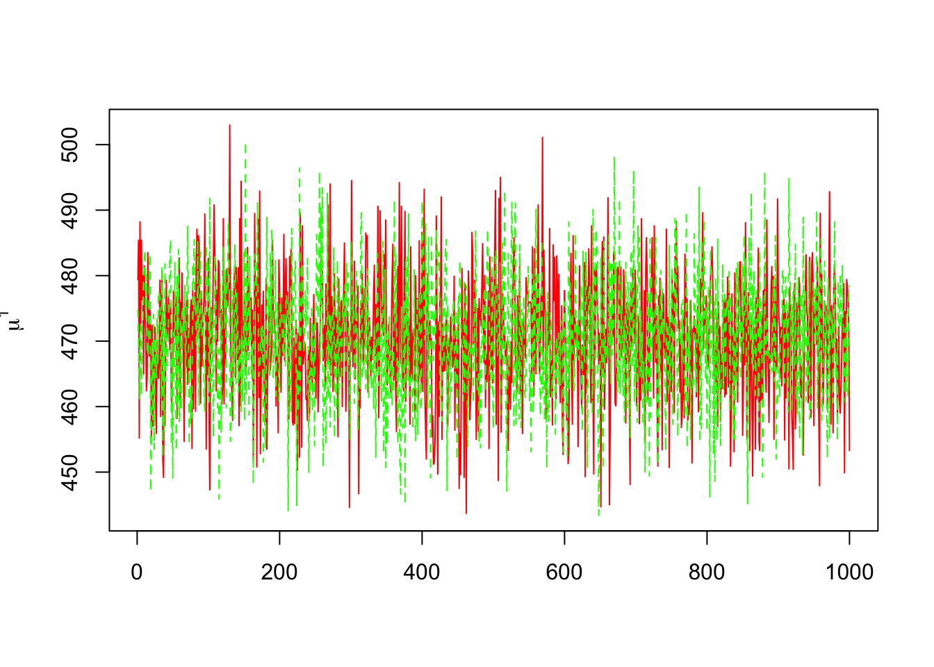
- Autocorrelation graph
> autocorr.diag(mu1)## [,1] [,2]
## Lag 0 1.00000000 1.000000000
## Lag 1 0.01556605 -0.005929771
## Lag 5 0.02089058 -0.027590187
## Lag 10 0.04427924 -0.018452354
## Lag 50 -0.08030862 0.002033798> autocorr.plot(mu1)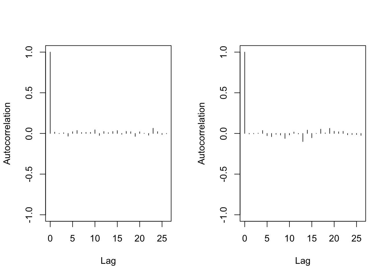
- We also compute a coefficient call \(\widehat{R}\) called The potential scale reduction factor. It is calculated for each estimated parametr, together with upper and lower confidence limits. Approximate convergence is diagnosed when the upper limit is close to 1. For multivariate chains, a multivariate value is calculated that bounds above the potential scale reduction factor for any linear combination of the (possibly transformed) variables.
\(\widehat{R}\) is greater than 1 and it declines to 1 when the number of iteration inscreases.
> gelman.diag(list(mu1[,1],mu1[,2]))## Potential scale reduction factors:
##
## Point est. Upper C.I.
## [1,] 1 1gelman.plot(list(mu1[,1],mu1[,2]))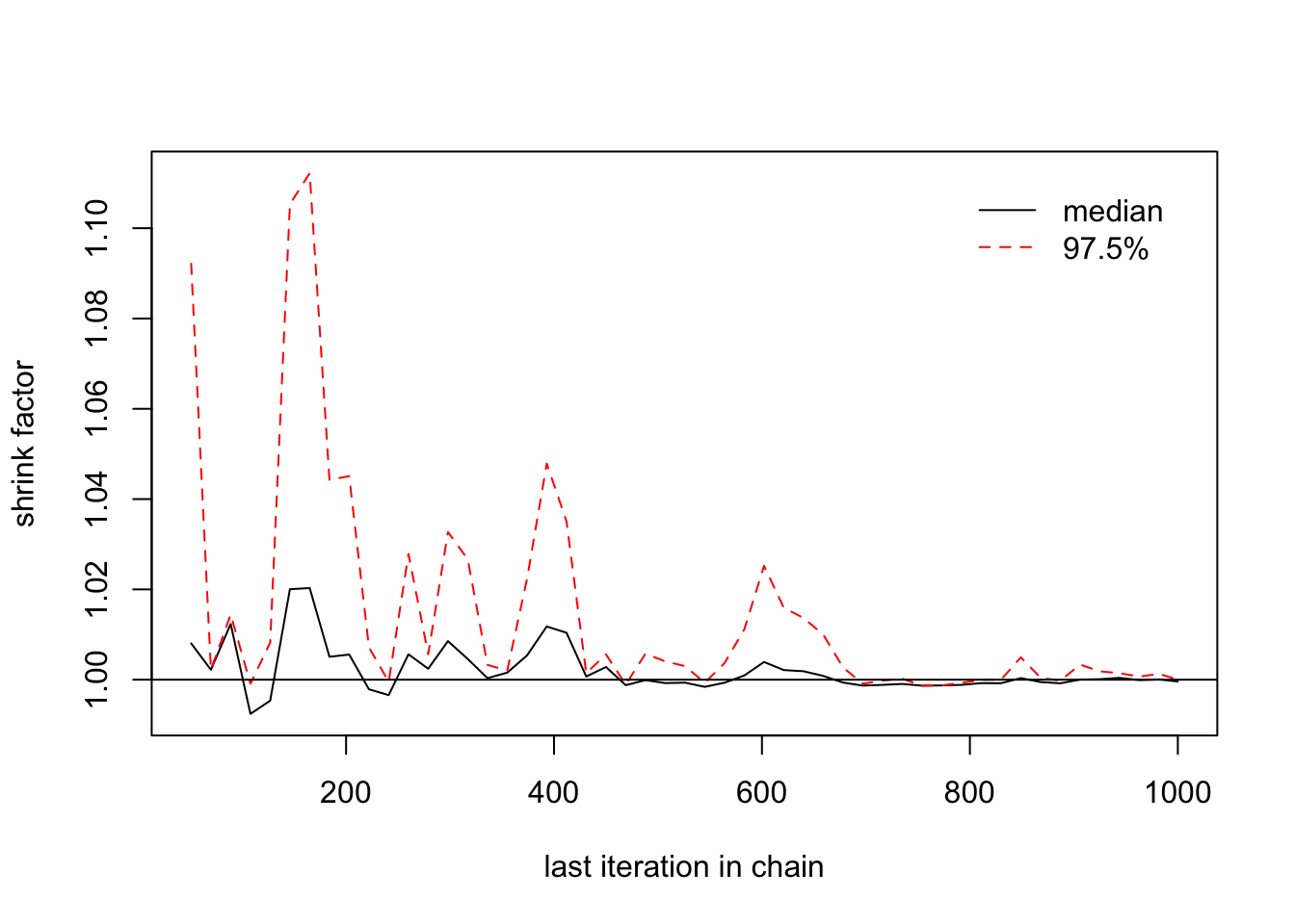
- Indeed \(\widehat{R}\) is expressed as follows:
\[\widehat{R}=\sqrt{\displaystyle\frac{\mbox{var}(\psi\mid y)}{W}}\] Where
\(\psi=\left(\psi\right)_{1\leq i\leq n,\; 1\leq j\leq m}\), \(n\) is the size of each Markov Chain, \(m\) is the number of Chains and \(\psi\) represents the estimated parameter.
\(W\) is the within variance : \[W=\displaystyle\frac{1}{m}\sum_{j=1}^m s_j^2\] where \[s^2_j=\displaystyle\frac{1}{n-1}\sum_{i=1}^n (\psi_{ij}-\overline{\psi}_{+ j})^2\]
\(\mbox{var}(\psi\mid y)\) is an average between the within and the between variances: \[\mbox{var}(\psi\mid y)=\displaystyle\frac{n-1}{n} W+\displaystyle\frac{B}{n}\] and where \[B=\displaystyle\frac{n}{m-1}\sum_{j=1}^m(\overline{\psi}_{+ j}-\overline{\psi}_{++})^2\]
Here \(\overline{\psi}_{++}\) and \(\overline{\psi}_{+ j}\) are averages computed on \(\psi\): \[\overline{\psi}_{+ j}=\displaystyle\frac{1}{n}\sum_{i=1}^n\psi_{ij}\] and \[\overline{\psi}_{++}=\displaystyle\frac{1}{m}\sum_{j=1}^m \overline{\psi}_{+ j}\]
Effictive sise of the sample: In the
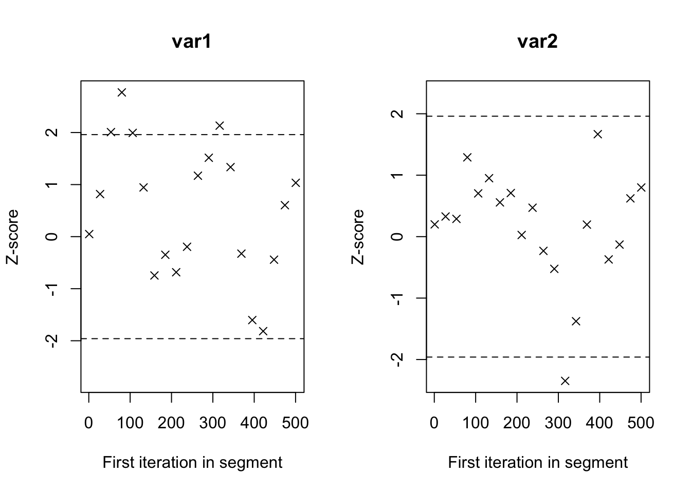
Routput of the commandbugsif the packageR2OpenBUGSwe give also an estimation of the effitive size of the Markov Chain that can been as the part of it where we had reached an independence and identically distributed sample with the posterior distribution. This effective size is then estimated as follows: \[ \widehat{\mbox{n.eff}}=\displaystyle\frac{nm}{1+2\sum_{t=1}^T\widehat{\rho}_t}\] where \(\widehat{\rho}_t\) is an estimation of the autocorrelation coefficient with lag \(t\) and \(T\) is the first odd positive integer for which \(\widehat{\rho}_{T+1}\) is negative.Geweke Diagnostics: It’s a diagnostic for Markov chains based on a test for equality of the means of the first and last part of a Markov chain (by default the first 10% and the last 50%). If the samples are drawn from the stationary distribution of the chain, the two means are equal and Geweke’s statistic has an asymptotically standard normal distribution.
The test statistic is a standard Z-score: the difference between the two sample means divided by its estimated standard error. The standard error is estimated from the spectral density at zero and so takes into account any autocorrelation.
> geweke.diag(mu1, frac1=0.1, frac2=0.5)##
## Fraction in 1st window = 0.1
## Fraction in 2nd window = 0.5
##
## var1 var2
## 0.04932 0.19942> geweke.plot(mu1, frac1=0.1, frac2=0.5)