Change Point Problem: Comparing three models

Introduction

I’m interesting in this Kernel in the comparison between three models and checking which of them is the best for the data.

I’m considering a very famous data set of annual counts of British coal mining disasters from 1851 to 1962.

> "CoalDisast" <-
+ structure(list(Year = as.integer(c(1851, 1852, 1853, 1854, 1855, 
+ 1856, 1857, 1858, 1859, 1860, 1861, 1862, 1863, 1864, 1865, 1866, 
+ 1867, 1868, 1869, 1870, 1871, 1872, 1873, 1874, 1875, 1876, 1877, 
+ 1878, 1879, 1880, 1881, 1882, 1883, 1884, 1885, 1886, 1887, 1888, 
+ 1889, 1890, 1891, 1892, 1893, 1894, 1895, 1896, 1897, 1898, 1899, 
+ 1900, 1901, 1902, 1903, 1904, 1905, 1906, 1907, 1908, 1909, 1910, 
+ 1911, 1912, 1913, 1914, 1915, 1916, 1917, 1918, 1919, 1920, 1921, 
+ 1922, 1923, 1924, 1925, 1926, 1927, 1928, 1929, 1930, 1931, 1932, 
+ 1933, 1934, 1935, 1936, 1937, 1938, 1939, 1940, 1941, 1942, 1943, 
+ 1944, 1945, 1946, 1947, 1948, 1949, 1950, 1951, 1952, 1953, 1954, 
+ 1955, 1956, 1957, 1958, 1959, 1960, 1961, 1962)), Count = c(4, 
+ 5, 4, 1, 0, 4, 3, 4, 0, 6, 3, 3, 4, 0, 2, 6, 3, 3, 5, 4, 5, 3, 
+ 1, 4, 4, 1, 5, 5, 3, 4, 2, 5, 2, 2, 3, 4, 2, 1, 3, 2, 2, 1, 1, 
+ 1, 1, 3, 0, 0, 1, 0, 1, 1, 0, 0, 3, 1, 0, 3, 2, 2, 0, 1, 1, 1, 
+ 0, 1, 0, 1, 0, 0, 0, 2, 1, 0, 0, 0, 1, 1, 0, 2, 3, 3, 1, 1, 2, 
+ 1, 1, 1, 1, 2, 4, 2, 0, 0, 0, 1, 4, 0, 0, 0, 1, 0, 0, 0, 0, 0, 
+ 1, 0, 0, 1, 0, 1)), .Names = c("Year", "Count"), row.names = c("1", 
+ "2", "3", "4", "5", "6", "7", "8", "9", "10", "11", "12", "13", 
+ "14", "15", "16", "17", "18", "19", "20", "21", "22", "23", "24", 
+ "25", "26", "27", "28", "29", "30", "31", "32", "33", "34", "35", 
+ "36", "37", "38", "39", "40", "41", "42", "43", "44", "45", "46", 
+ "47", "48", "49", "50", "51", "52", "53", "54", "55", "56", "57", 
+ "58", "59", "60", "61", "62", "63", "64", "65", "66", "67", "68", 
+ "69", "70", "71", "72", "73", "74", "75", "76", "77", "78", "79", 
+ "80", "81", "82", "83", "84", "85", "86", "87", "88", "89", "90", 
+ "91", "92", "93", "94", "95", "96", "97", "98", "99", "100", 
+ "101", "102", "103", "104", "105", "106", "107", "108", "109", 
+ "110", "111", "112"), class = "data.frame")
> head(CoalDisast)

##   Year Count
## 1 1851     4
## 2 1852     5
## 3 1853     4
## 4 1854     1
## 5 1855     0
## 6 1856     4

When plotting the time-series graph (see below) we can notice that the curve decreases around the year 1900. So we may think that there’s a change of the model sometime around 1900. Since the observed data is a count data, we may think that it’s better to consider a Poisson probability distribution to model the observed count.

Then if we think that there’s no change of the number of accident, the best model could be: \[\forall\,i=,\ldots,n,\;\; D[i]~\mbox{Poisson}(\lambda)\] where \(D\) is the vector of number of Disasters between 1850 to 1962.

If we think that there’s one change point in the model we will consider that the best model of the data is the following \[\forall\,i=1,\ldots,\tau,\;\; D[i]\sim\mbox{Poisson}(\lambda_1)\] and \[\forall\,i=\tau+1,\ldots,n,\;\; D[i]\sim\mbox{Poisson}(\lambda_2)\] where \(\tau\) is the change-point that should be estimated.

Finally the last model that will considered here is a Model with two change-points

\[\forall\,i=1,\ldots,\tau_1,\;\; D[i]~\mbox{Poisson}(\lambda_1),\] \[\forall\,i=\tau_1+1,\ldots,\tau_2,\;\; D[i]\sim\mbox{Poisson}(\lambda_2)\] and \[\forall\,i=\tau_2+1,\ldots,n,\;\; D[i]\sim\mbox{Poisson}(\lambda_3)\]

The aim of this Kernel will be then to estimate these three models using a Bayesian Approach, running them using R2OpenBUGS, making an exhaustive diagnostic of their convergence and comparing between three models and answer to the questions: Is there any significant change-point in the data? If this change-point exists, is it only or more than 2?

The Models

Since we have no prior information on the parameters we will use in the three cases non-informative priors.

Here’s below the BUGS code of the three models:

Model without change point

model{
  for (year in 1:N) {
    D[year] ~ dpois(mu[year])
    log(mu[year]) <- b
  }
  b~ dnorm(0.0, 1.0E-6) 
}

Model with one change point

 model {
    for (year in 1:N) {
    D[year] ~ dpois(mu[year])
    log(mu[year]) <- b[1] + step(year - changeyear) * b[2]
    }
    for (j in 1:2) { b[j] ~ dnorm(0.0, 1.0E-6) }
    changeyear ~ dunif(1,N)
    }

Model with two change points

 model {
    for (year in 1:N) {
      D[year] ~ dpois(mu[year])
      log(mu[year]) <- b[1] + step(year - changeyear) * b[2]+ step(year-(changeyear+delta))*b[3]
    }
    for (j in 1:3) { b[j] ~ dnorm(0.0, .01) }
    
    changeyear ~ dunif(1,N)
    delta1 ~ dunif(1,N)
    delta<- delta1*step(N-(changeyear+delta1))
  }

`R` implementation

As mentioned above we will use for this analysis R2OpenBUGS, we need then to write these three models into three different .txt files. We need to write three R functions to initialize the Markov Chains. Here’s then the R code that should implemented. We will later run the bugs command and study the convergence of each Markov Chain.

Let’s first load the needed packages

> library(R2OpenBUGS)
> library(coda)

The initializing functions

> inits0<-function(){
+   inits=list(b=rnorm(1))
+ }
> 
> inits1<-function(){
+   inits=list(b=rnorm(2),changeyear=3)
+ }
> 
> inits1<-function(){
+   inits=list(b=rnorm(3),changeyear=3,delta=3)
+ }

The parameters

> params0<-"b"
> 
> param1<-c("b","changeyear")
> 
> param2<-c("b","changeyear","delta")

Creating the files of the BUGS code

###  Model0
sink("Mod0_cp.txt")
cat("
model{
  for (year in 1:N) {
    D[year] ~ dpois(mu[year])
    log(mu[year]) <- b
    }
    b~ dnorm(0.0, 1.0E-6) 
    }
    ",fill=T)
sink()

### Model1

sink("Mod1_cp.txt")
cat("
model {
    for (year in 1:N) {
    D[year] ~ dpois(mu[year])
    log(mu[year]) <- b[1] + step(year - changeyear) * b[2]
    }
    for (j in 1:2) { b[j] ~ dnorm(0.0, 1.0E-6) }
    changeyear ~ dunif(1,N)
    }
    ",fill=T)
sink()


###  Model2
sink("Mod2_cp.txt")
cat("model {
  for (year in 1:N) {
    D[year] ~ dpois(mu[year])
    log(mu[year]) <- b[1] + step(year - changeyear) * b[2]+ step(year-(changeyear+delta))*b[3]
  }
  for (j in 1:3) { b[j] ~ dnorm(0.0, .01) }
  
  changeyear ~ dunif(1,N)
  delta1 ~ dunif(1,N)
  delta<- delta1*step(N-(changeyear+delta1))
}
",fill=T)
sink()

filename0<-"Mod0_cp.txt"
filename1<-"Mod1_cp.txt"
filename2<-"Mod2_cp.txt"

Running now the Markov Chains (if you use MAC OS). We will run three MC with 10,000 iterations with a burn-in equal to 9000.

out0<-bugs(dt,inits0,params0,filename0,codaPkg=F,n.burnin = 9000,
     n.thin =1, n.iter=10000,debug=F,
     n.chains = 3,working.directory=getwd(),
     OpenBUGS.pgm=OpenBUGS.pgm, useWINE=T)
out1<-bugs(dt,inits1,params1,filename1,codaPkg=F,
     n.thin =1, n.iter=10000,debug=F,
     n.chains = 3,working.directory=getwd(),
     OpenBUGS.pgm=OpenBUGS.pgm2, useWINE=T)
out2<-bugs(dt,inits2,params2,filename2,codaPkg=F,
     n.thin =1, n.iter=10000,debug=F,
     n.chains = 3,working.directory=getwd(),
     OpenBUGS.pgm=OpenBUGS.pgm, useWINE=T)

Diagonostic of the Models

Model without change-point

We will then check the convergence of the Markov Chain contained in the R out0.

We start then by the trace plot of the parameters

> dim(out0$sims.array)

## [1] 1000    3    2

> b=mcmc(out0$sims.array[,,1])
> lambda=exp(b)
> matplot(lambda,col=c("red","green","blue"),ylab=expression(lambda),type="l")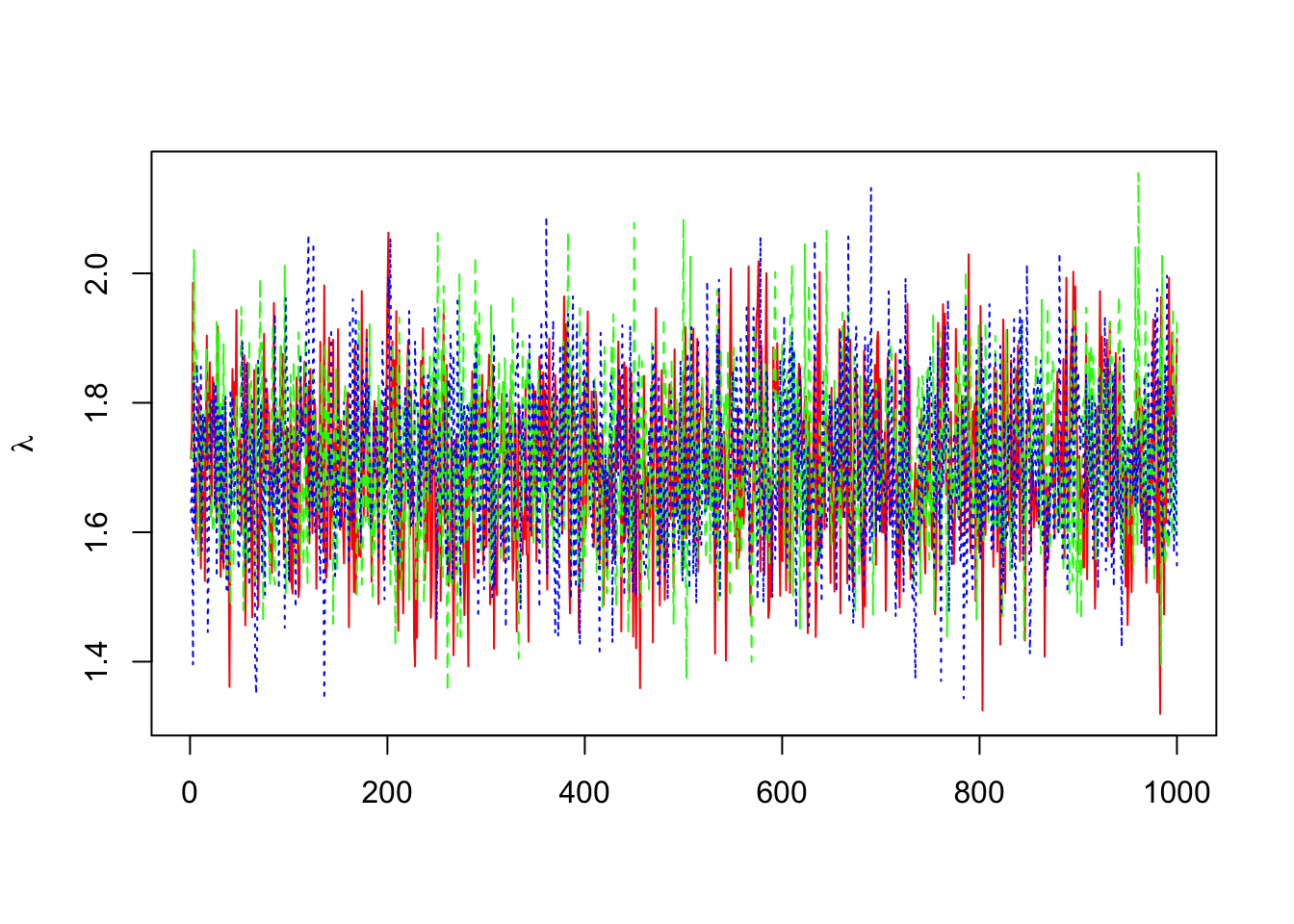

We proceed also by estimating the \(widehat{R}\) and its confidence interval:

> gelman.diag(list(b[,1],b[,2],b[,3]))

## Potential scale reduction factors:
## 
##      Point est. Upper C.I.
## [1,]          1          1

> gelman.plot(list(b[,1],b[,2],b[,3]))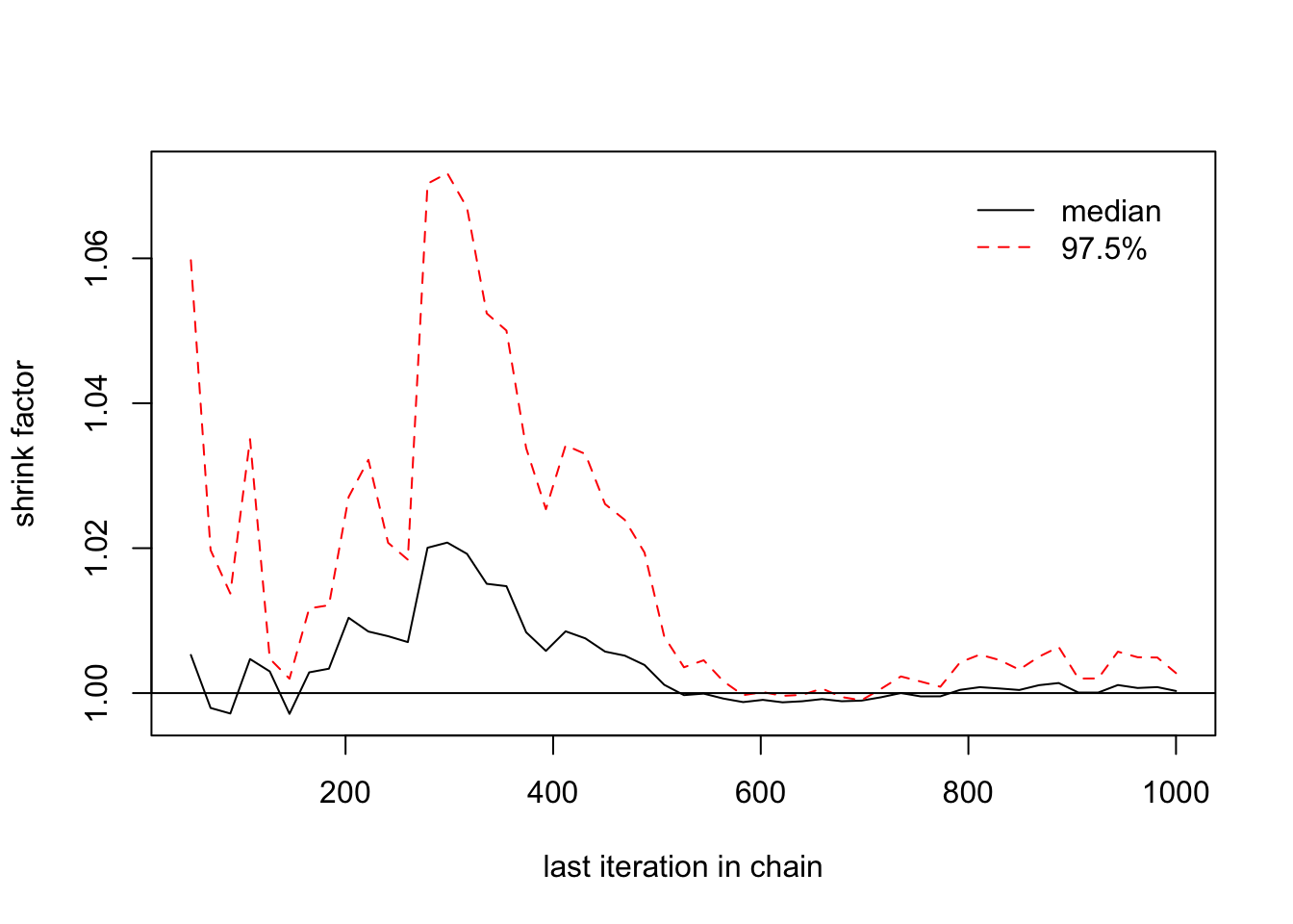

Let us proceed to the auto-correlation diagnostics

> autocorr(b)

## , , 1
## 
##               [,1]         [,2]         [,3]
## Lag 0  1.000000000  0.034495282  0.009053795
## Lag 1  0.055236668  0.005261091  0.032532027
## Lag 5  0.004546683 -0.041912206  0.030566490
## Lag 10 0.014320159  0.007779867 -0.012681079
## Lag 50 0.022827788  0.028042545 -0.004772002
## 
## , , 2
## 
##                [,1]         [,2]          [,3]
## Lag 0   0.034495282  1.000000000 -0.0653159430
## Lag 1  -0.019183478  0.010794786 -0.0381613522
## Lag 5  -0.042394955  0.007569832  0.0446293938
## Lag 10  0.037666659 -0.032733381 -0.0007449515
## Lag 50  0.003538836 -0.001874355 -0.0376931809
## 
## , , 3
## 
##                [,1]         [,2]         [,3]
## Lag 0   0.009053795 -0.065315943  1.000000000
## Lag 1   0.026839667 -0.009128083  0.023306859
## Lag 5  -0.005668425  0.023113228  0.004772442
## Lag 10 -0.011456955 -0.017848935 -0.001289498
## Lag 50  0.004717675 -0.043223337  0.027772753

> autocorr.diag(b,0:10)

##                [,1]          [,2]         [,3]
## Lag 0   1.000000000  1.0000000000  1.000000000
## Lag 1   0.055236668  0.0107947855  0.023306859
## Lag 2   0.001513254 -0.0339514475 -0.006365209
## Lag 3  -0.026223719 -0.0733879404  0.028001594
## Lag 4   0.037489899  0.0411621092 -0.044719691
## Lag 5   0.004546683  0.0075698318  0.004772442
## Lag 6  -0.045736486 -0.0001354907  0.061712056
## Lag 7  -0.014715923 -0.0039889180 -0.013845836
## Lag 8  -0.019906335  0.0046344412  0.039821934
## Lag 9  -0.065611560 -0.0473617932 -0.007516563
## Lag 10  0.014320159 -0.0327333815 -0.001289498

> n<-nrow(b)
> cor(b[-n,1],b[-1,1])

## [1] 0.05530207

> cor(b[-c(n:(n-1)),1],b[-c(1,2),1])

## [1] 0.001514258

> autocorr.plot(b)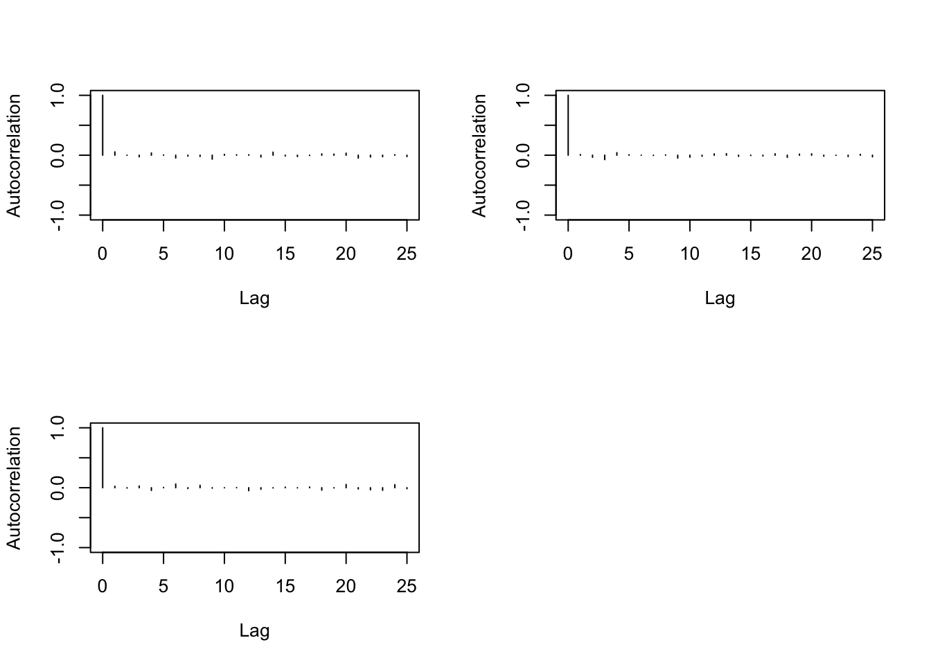

We finally proceed to the Geweke diagnostics that show the stationary of the generated sample.

> geweke.diag(b)

## 
## Fraction in 1st window = 0.1
## Fraction in 2nd window = 0.5 
## 
##     var1     var2     var3 
## -0.05311  0.06627 -1.26129

We can then decide here to the convergence of the generated Markov Chain in the Model without considering any change-point.

Model with one change-point

We will then check the convergence of the Markov Chain contained in the R out1.

We start then by the trace plot of the parameters

> dim(out1$sims.array)
## [1] 1000    3    4
> b1=mcmc(out1$sims.array[,,1])
> lambda1=exp(b1)
> matplot(lambda1,col=c("red","green","blue"),type="l")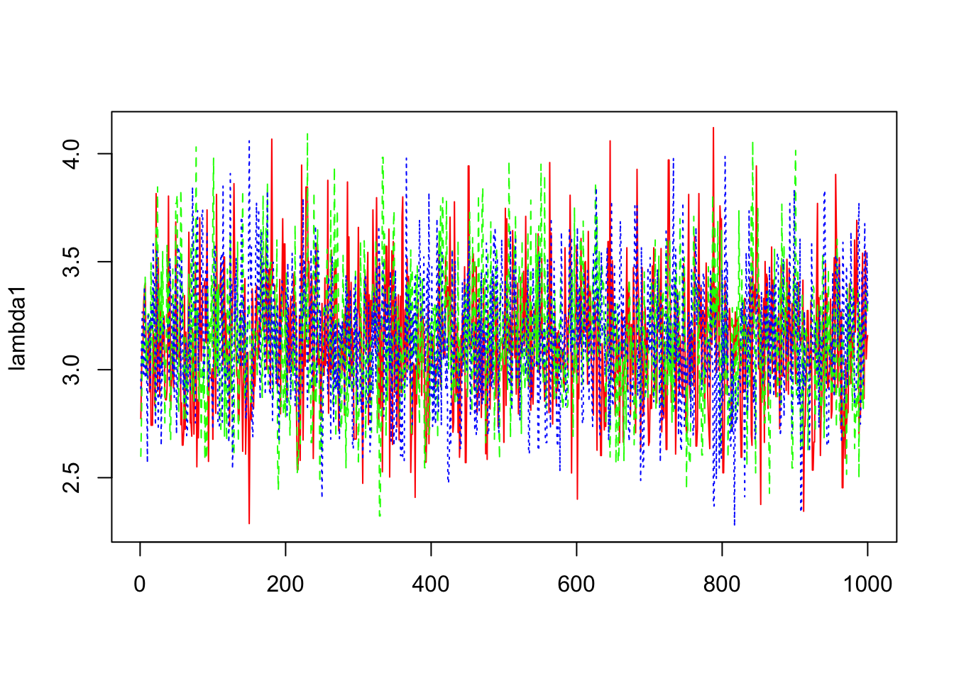

> 
> b2=mcmc(out1$sims.array[,,2])
> lambda2=exp(b1+b2)
> matplot(lambda2,col=c("red","green","blue"),type="l")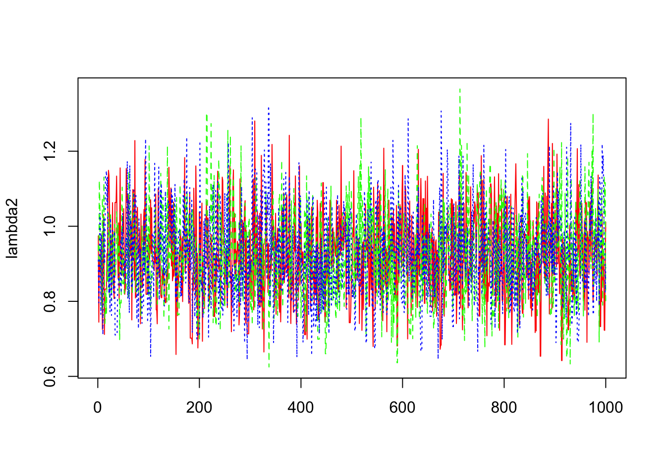

> 
> 
> changeyear=mcmc(out1$sims.array[,,3])
> matplot(changeyear,col=c("red","green","blue"),type="l")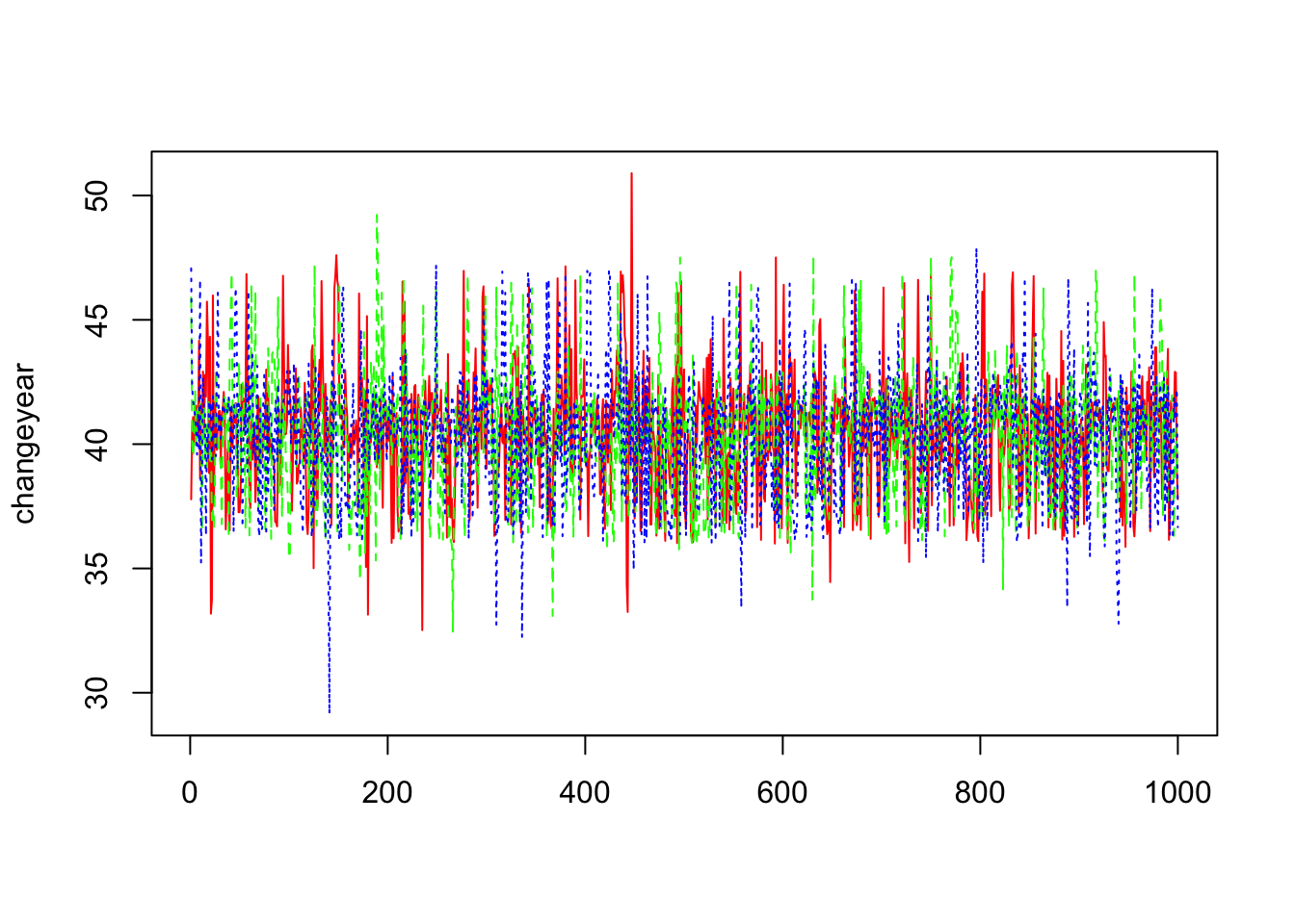

We can’t then conclude from these trace plots any abnormality in the convergence of the Markov Chain and let us then proceed to the others diagnostic methods.

Estimation of \(\widehat{R}\)

> gelman.diag(list(b1[,1],b1[,2],b1[,3]))
## Potential scale reduction factors:
## 
##      Point est. Upper C.I.
## [1,]          1          1
> gelman.plot(list(b1[,1],b1[,2],b1[,3]))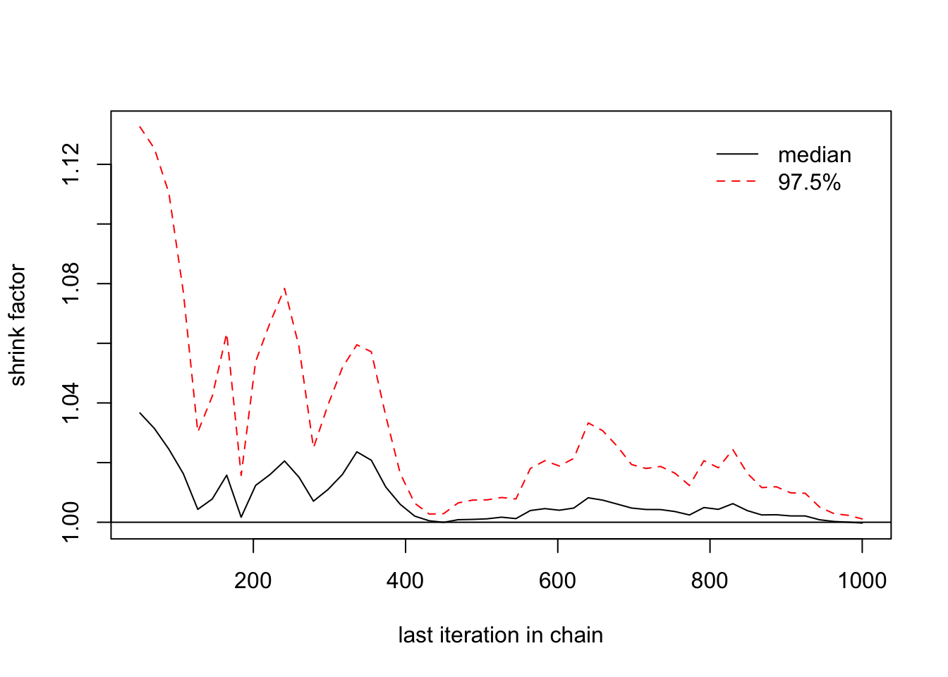

> 
> gelman.diag(list(b2[,1],b2[,2],b2[,3]))
## Potential scale reduction factors:
## 
##      Point est. Upper C.I.
## [1,]          1          1
> gelman.plot(list(b2[,1],b2[,2],b2[,3]))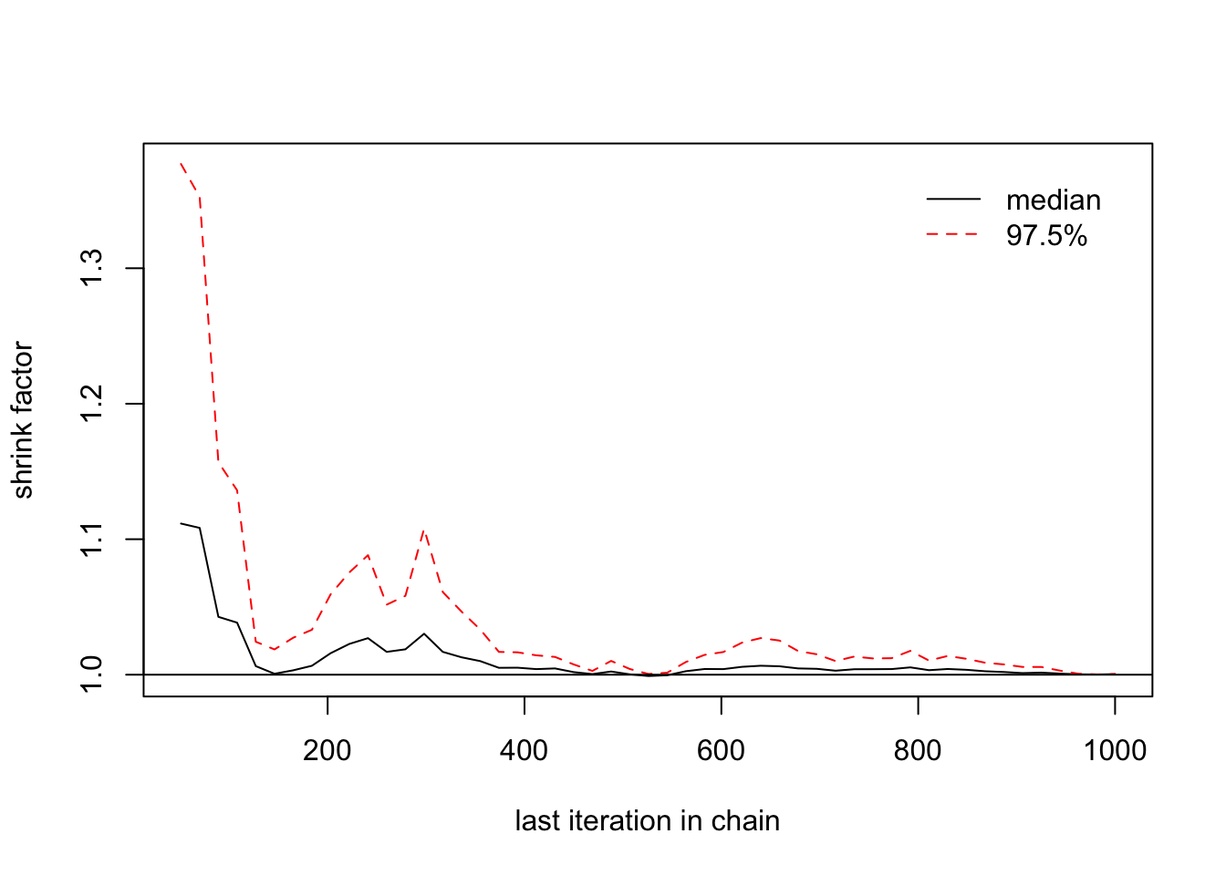

> 
> gelman.diag(list(changeyear[,1],changeyear[,2],changeyear[,3]))
## Potential scale reduction factors:
## 
##      Point est. Upper C.I.
## [1,]          1          1
> gelman.plot(list(changeyear[,1],changeyear[,2],changeyear[,3])) ## We need a longer MC

We may need to run the MC with a number of iterations longer than 10,000

Auto-correlation procedure

> autocorr.diag(b1,0:10)
##               [,1]         [,2]         [,3]
## Lag 0   1.00000000  1.000000000  1.000000000
## Lag 1   0.24267721  0.230358879  0.266753010
## Lag 2   0.07057706  0.092150937  0.045069049
## Lag 3   0.01995826  0.067175082  0.031460518
## Lag 4  -0.02823631  0.029342496  0.056167906
## Lag 5  -0.01962895 -0.005534525 -0.026834848
## Lag 6   0.02084450  0.034985551 -0.013646786
## Lag 7  -0.03542723  0.005210021  0.024432555
## Lag 8  -0.04131954  0.020949803 -0.015066116
## Lag 9  -0.05499395  0.010438041  0.005232191
## Lag 10  0.01825271 -0.051816493  0.026413601
> autocorr.plot(b1)

> 
> autocorr.diag(b2,0:10)
##                 [,1]         [,2]         [,3]
## Lag 0   1.0000000000  1.000000000  1.000000000
## Lag 1   0.2569770523  0.220929046  0.240071995
## Lag 2   0.0753613247  0.110964052  0.077083558
## Lag 3   0.0547489236 -0.006831899  0.054980560
## Lag 4   0.0170650988 -0.003856126  0.056993255
## Lag 5  -0.0287166286 -0.004394506  0.002354384
## Lag 6  -0.0197918237 -0.014834011 -0.040336202
## Lag 7   0.0331368353  0.026915925  0.017319707
## Lag 8   0.0007594842  0.076272581 -0.022211247
## Lag 9   0.0437559858  0.008575427 -0.022689286
## Lag 10  0.0156435436 -0.058137191 -0.003824708
> autocorr.plot(b2)

> 
> autocorr.diag(changeyear,0:10)
##                [,1]         [,2]         [,3]
## Lag 0   1.000000000  1.000000000  1.000000000
## Lag 1   0.150604976  0.206223983  0.201395628
## Lag 2   0.090038275  0.047625876  0.075335272
## Lag 3   0.029118126  0.014947818 -0.011368724
## Lag 4  -0.014583715  0.032821822 -0.054976051
## Lag 5  -0.019055907  0.068669698 -0.041180419
## Lag 6  -0.024874577  0.043309950 -0.109348407
## Lag 7  -0.001704167  0.037493443 -0.069400442
## Lag 8   0.032943349  0.034910472 -0.006312559
## Lag 9  -0.038963690  0.035209870  0.002263666
## Lag 10  0.022007605 -0.008365255  0.003941313
> autocorr.plot(changeyear)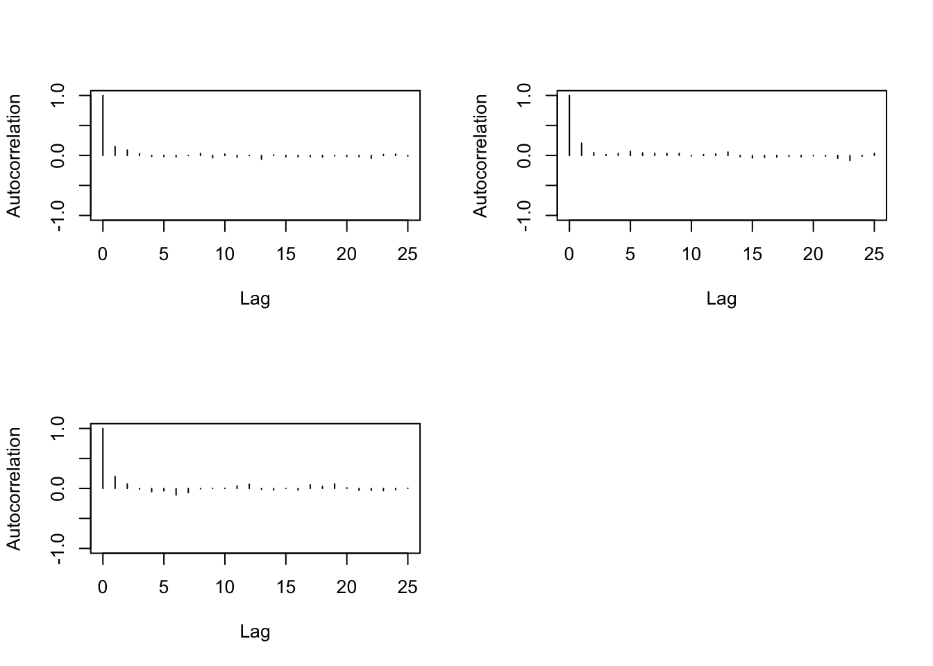

We need then to increase the thin when running the MC.

a new update of the MC:

Let us then proceed for another convergence diagnostics:

> 
> b1=mcmc(out1$sims.array[,,1])
> b2=mcmc(out1$sims.array[,,2])
> changeyear=mcmc(out1$sims.array[,,3])
> 
> gelman.diag(list(b1[,1],b1[,2],b1[,3]))
## Potential scale reduction factors:
## 
##      Point est. Upper C.I.
## [1,]          1          1
> gelman.plot(list(b1[,1],b1[,2],b1[,3]))

> 
> gelman.diag(list(b2[,1],b2[,2],b2[,3]))
## Potential scale reduction factors:
## 
##      Point est. Upper C.I.
## [1,]          1          1
> gelman.plot(list(b2[,1],b2[,2],b2[,3]))

> 
> gelman.diag(list(changeyear[,1],changeyear[,2],changeyear[,3]))
## Potential scale reduction factors:
## 
##      Point est. Upper C.I.
## [1,]          1          1
> gelman.plot(list(changeyear[,1],changeyear[,2],changeyear[,3])) ## We need a longer MC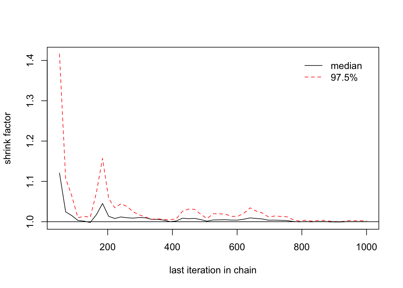

> autocorr.diag(b1,0:10)
##               [,1]         [,2]         [,3]
## Lag 0   1.00000000  1.000000000  1.000000000
## Lag 1   0.24267721  0.230358879  0.266753010
## Lag 2   0.07057706  0.092150937  0.045069049
## Lag 3   0.01995826  0.067175082  0.031460518
## Lag 4  -0.02823631  0.029342496  0.056167906
## Lag 5  -0.01962895 -0.005534525 -0.026834848
## Lag 6   0.02084450  0.034985551 -0.013646786
## Lag 7  -0.03542723  0.005210021  0.024432555
## Lag 8  -0.04131954  0.020949803 -0.015066116
## Lag 9  -0.05499395  0.010438041  0.005232191
## Lag 10  0.01825271 -0.051816493  0.026413601
> autocorr.plot(b1)

> 
> autocorr.diag(b2,0:10)
##                 [,1]         [,2]         [,3]
## Lag 0   1.0000000000  1.000000000  1.000000000
## Lag 1   0.2569770523  0.220929046  0.240071995
## Lag 2   0.0753613247  0.110964052  0.077083558
## Lag 3   0.0547489236 -0.006831899  0.054980560
## Lag 4   0.0170650988 -0.003856126  0.056993255
## Lag 5  -0.0287166286 -0.004394506  0.002354384
## Lag 6  -0.0197918237 -0.014834011 -0.040336202
## Lag 7   0.0331368353  0.026915925  0.017319707
## Lag 8   0.0007594842  0.076272581 -0.022211247
## Lag 9   0.0437559858  0.008575427 -0.022689286
## Lag 10  0.0156435436 -0.058137191 -0.003824708
> autocorr.plot(b2)

> 
> autocorr.diag(changeyear,0:10)
##                [,1]         [,2]         [,3]
## Lag 0   1.000000000  1.000000000  1.000000000
## Lag 1   0.150604976  0.206223983  0.201395628
## Lag 2   0.090038275  0.047625876  0.075335272
## Lag 3   0.029118126  0.014947818 -0.011368724
## Lag 4  -0.014583715  0.032821822 -0.054976051
## Lag 5  -0.019055907  0.068669698 -0.041180419
## Lag 6  -0.024874577  0.043309950 -0.109348407
## Lag 7  -0.001704167  0.037493443 -0.069400442
## Lag 8   0.032943349  0.034910472 -0.006312559
## Lag 9  -0.038963690  0.035209870  0.002263666
## Lag 10  0.022007605 -0.008365255  0.003941313
> autocorr.plot(changeyear)

> geweke.diag(b1)
## 
## Fraction in 1st window = 0.1
## Fraction in 2nd window = 0.5 
## 
##    var1    var2    var3 
## -1.3211  0.7069  1.0024
> geweke.diag(b2)
## 
## Fraction in 1st window = 0.1
## Fraction in 2nd window = 0.5 
## 
##    var1    var2    var3 
##  1.6899 -0.8169 -0.9576
> geweke.diag(changeyear)
## 
## Fraction in 1st window = 0.1
## Fraction in 2nd window = 0.5 
## 
##    var1    var2    var3 
## 0.01496 0.47468 2.24082

The later MC convergences then and it can be considered that contains a good estimation of the posterior distribution.

Model with two change-points

We can already notice that the pD is negative

> out2$pD
## [1] -10.83

It’s know that this means that either there’s a conflict between the likelihood and the prior (bad choice for the prior) or the posterior mean is a poor estimator of the parameters. This model has to be rejected.

Finally when comparing the DIC of the two accepted models

> out1a$DIC
## [1] 344.1
> out0$DIC
## [1] 409.8

We can conclude that the model with one change-point fits better the data. We conclude that the mean of the number of disasters was following a Poisson distribution with mean

> exp(mean(out1a$sims.array[,,1]))
## [1] 3.108822

before the year

> round(mean(out1a$sims.array[,,3])+1850)
## [1] 1890

This change happened with a probability 95% between the years

> round(quantile(out1a$sims.array[,,3],probs = c(0.025,0.975))+1850)
##  2.5% 97.5% 
##  1886  1896

After this change-point the distribution of the number of disasters is a Poisson distribution with mean

> exp(mean(out1a$sims.array[,,1]+out1a$sims.array[,,2]))
## [1] 0.9141008