R
Gibbs sampler
What’s a Gibbs Sampler
It’s an algorithm for simulating Markov chains.
Let \(\theta=(\theta_1,\ldots,\theta_k)\) be a random vector with joint distribution \(f\),
Aim: simulate a sample with distribution \(f\).
How it works?
Choose arbitrary starting values: \(\theta^{(0)}=(\theta_1^{(0)},\ldots,\theta_k^{(0)})\)
Sample new values for each element of \(\theta\) by cycling through the following steps:
Sample a new value for \(\theta_1^{(1)}\) from the full conditional distribution of \(\theta_1\) given the most recent values of all other elements of \(\theta\): \[ \theta_1^{(1)}\sim p\left(\theta_1 \mid\theta_2^{(0)},\ldots,\theta_k^{(0)} \right)\]
Sample a new value \(\theta_2^{(1)}\) for the 2nd component of \(\theta\), from its full conditional distribution \[ \theta_2^{(1)}\sim p\left(\theta_2 \mid\theta_1^{(1)},\theta_3^{(0)}\ldots,\theta_k^{(0)} \right)\]
- …
\(\theta_k^{(1)}\sim p\left(\theta_1 \mid\theta_1^{(1)},\theta_2^{(1)}\ldots,\theta_{k-1}^{(1)} \right)\)
This completes one iteration of the Gibbs sampler and generates a new realization of the vector of unknowns \(\theta^{(1)}\).
- Repeat Step 2 many times and obtain a sample \(\theta^{(1)},\ldots, \theta^{(T)}\)
To better understand the Gibbs Sampler, I suggest to read the paper by Casela and George 1992
Markov Chain
\(\theta^{(1)},\ldots, \theta^{(T)}\) is a Markov Chain
If \(\theta^{(1)},\ldots, \theta^{(T)}\) converges, then from \(N\), \(\theta^{(N)},\ldots, \theta^{(N)}\) is a sample with \(f\) distribution
codaandcodadiagstwoRpackages for convergence diagnostics
Example 1: Posterior of the couple mean and precision of a Normal distribution
Problem
Suppose that we had observed a sample \(y_1,\ldots,y_n\) generated from random variable \(Y\sim\mathcal{N}\left(\mbox{mean}=\mu,\,\mbox{Var}=1/\tau\right)\) where \(\mu\) and \(\tau\) are unknown. Suppose also that we had defined the following prior distribution \[f(\mu,\,\tau) \propto 1/\tau\]
Based on a sample, obtain the posterior distributions of \(\mu\) and \(\tau\) using the Gibbs sampler and write an R code simulating this posterior distribution.
Solution
We can first prouve that
- Conditional posterior for the mean, given the precision is given by
\[\mu\mid y_1,\ldots,y_n,\tau \sim \mathcal{N}\left(\overline{y},\displaystyle\frac{1}{n\tau}\right)\]
- Conditional posterior for the precision, given the mean
\[\tau\mid y_1,\ldots,y_n,\mu \sim \mbox{Gamma}\left(\displaystyle\frac{n}{2},\displaystyle\frac{2}{(n-1)s^2+n(\mu-\overline{y})^2}\right)\] where \[\overline{y}=\displaystyle\frac{1}{n}\sum_{i=1}^n y_i\] is the sample mean and \[s^2=\displaystyle\frac{1}{n-1}\sum_{i=1}^n (y_i-\overline{y})^2\] is the sample variance.
Let’s then implement then the Gibbs Sampler into R. Here’s the code
> # The data
> n    <- 40
> ybar <- 35
> s2   <- 5
>
> # sample from the joint posterior (mu, tau | data)
> mu     <- rep(NA, 11000)
> tau    <- rep(NA, 11000)
> T      <- 1000    # burnin
> tau[1] <- 1  # initialisation
> mu[1] <- 1
> for(i in 2:11000) {
+     mu[i]  <- rnorm(n = 1, mean = ybar, sd = sqrt(1 / (n * tau[i - 1])))
+     tau[i] <- rgamma(n = 1, shape = n / 2, scale = 2 / ((n - 1) * s2 + n * (mu[i] - ybar)^2))
+ }
> mu  <- mu[-(1:T)]   # remove burnin
> tau <- tau[-(1:T)] # remove burnin
Let’s quickly visualize the marginal distribution obtained from the sample runned above.
> summary(mu) Min. 1st Qu. Median Mean 3rd Qu. Max.
33.66 34.75 35.00 35.00 35.24 36.49 > hist(mu)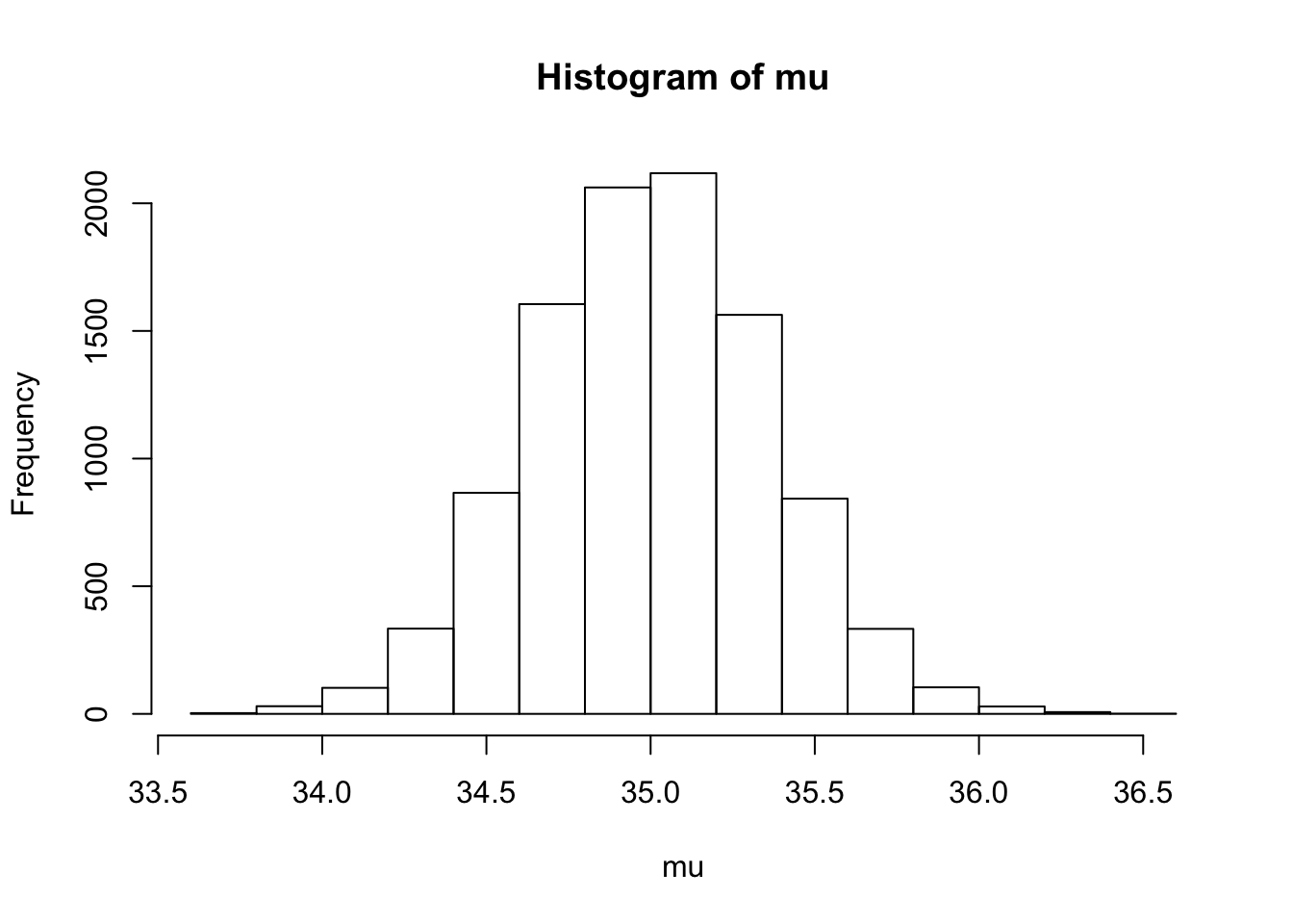
> summary(1/tau) Min. 1st Qu. Median Mean 3rd Qu. Max.
2.364 4.353 5.061 5.241 5.934 13.035 > hist(1/tau)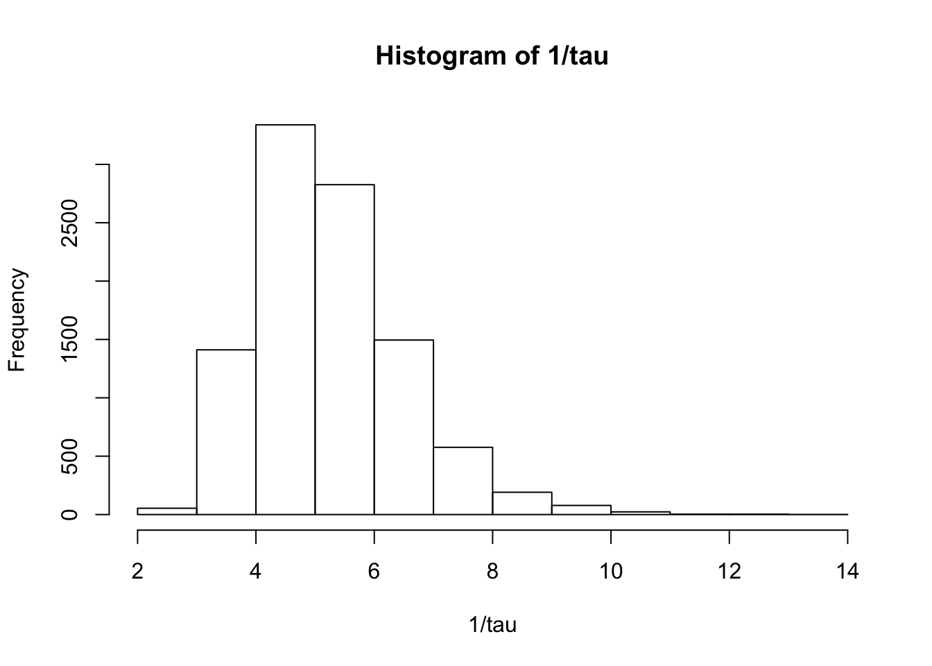
Example 2: Bivariate Gaussian Distribution
Let \[\theta=(\theta_1,\,\theta_2)\sim \mathcal{N}_2(0,I_2)\] with density function \[f(\theta_1,\,\theta_2)=\displaystyle\frac{1}{\sqrt{2\pi}}\exp\left(-\displaystyle\frac{1}{2}(\theta_1^2+\theta_2^2)\right)\]
Compute the distributions of \(\theta_1 \mid \theta_2\) and \(\theta_2 \mid \theta_1\)
Write an
Rcode based on the Gibbs algorithm to simulate a sample with a Standard bivariate Gaussian distribution.