The Bayesian Model
Consider the data set of annual counts of British coal mining disasters from 1851 to 1962.
> "CoalDisast" <-
+ structure(list(Year = as.integer(c(1851, 1852, 1853, 1854, 1855,
+ 1856, 1857, 1858, 1859, 1860, 1861, 1862, 1863, 1864, 1865, 1866,
+ 1867, 1868, 1869, 1870, 1871, 1872, 1873, 1874, 1875, 1876, 1877,
+ 1878, 1879, 1880, 1881, 1882, 1883, 1884, 1885, 1886, 1887, 1888,
+ 1889, 1890, 1891, 1892, 1893, 1894, 1895, 1896, 1897, 1898, 1899,
+ 1900, 1901, 1902, 1903, 1904, 1905, 1906, 1907, 1908, 1909, 1910,
+ 1911, 1912, 1913, 1914, 1915, 1916, 1917, 1918, 1919, 1920, 1921,
+ 1922, 1923, 1924, 1925, 1926, 1927, 1928, 1929, 1930, 1931, 1932,
+ 1933, 1934, 1935, 1936, 1937, 1938, 1939, 1940, 1941, 1942, 1943,
+ 1944, 1945, 1946, 1947, 1948, 1949, 1950, 1951, 1952, 1953, 1954,
+ 1955, 1956, 1957, 1958, 1959, 1960, 1961, 1962)), Count = c(4,
+ 5, 4, 1, 0, 4, 3, 4, 0, 6, 3, 3, 4, 0, 2, 6, 3, 3, 5, 4, 5, 3,
+ 1, 4, 4, 1, 5, 5, 3, 4, 2, 5, 2, 2, 3, 4, 2, 1, 3, 2, 2, 1, 1,
+ 1, 1, 3, 0, 0, 1, 0, 1, 1, 0, 0, 3, 1, 0, 3, 2, 2, 0, 1, 1, 1,
+ 0, 1, 0, 1, 0, 0, 0, 2, 1, 0, 0, 0, 1, 1, 0, 2, 3, 3, 1, 1, 2,
+ 1, 1, 1, 1, 2, 4, 2, 0, 0, 0, 1, 4, 0, 0, 0, 1, 0, 0, 0, 0, 0,
+ 1, 0, 0, 1, 0, 1)), .Names = c("Year", "Count"), row.names = c("1",
+ "2", "3", "4", "5", "6", "7", "8", "9", "10", "11", "12", "13",
+ "14", "15", "16", "17", "18", "19", "20", "21", "22", "23", "24",
+ "25", "26", "27", "28", "29", "30", "31", "32", "33", "34", "35",
+ "36", "37", "38", "39", "40", "41", "42", "43", "44", "45", "46",
+ "47", "48", "49", "50", "51", "52", "53", "54", "55", "56", "57",
+ "58", "59", "60", "61", "62", "63", "64", "65", "66", "67", "68",
+ "69", "70", "71", "72", "73", "74", "75", "76", "77", "78", "79",
+ "80", "81", "82", "83", "84", "85", "86", "87", "88", "89", "90",
+ "91", "92", "93", "94", "95", "96", "97", "98", "99", "100",
+ "101", "102", "103", "104", "105", "106", "107", "108", "109",
+ "110", "111", "112"), class = "data.frame")
> head(CoalDisast)
## Year Count
## 1 1851 4
## 2 1852 5
## 3 1853 4
## 4 1854 1
## 5 1855 0
## 6 1856 4- Let us look at the data and see the evolution of the number of disasters.
library(ggplot2)
p<-ggplot(CoalDisast,aes(x=Year,y=Count))+geom_line()+theme_bw()
p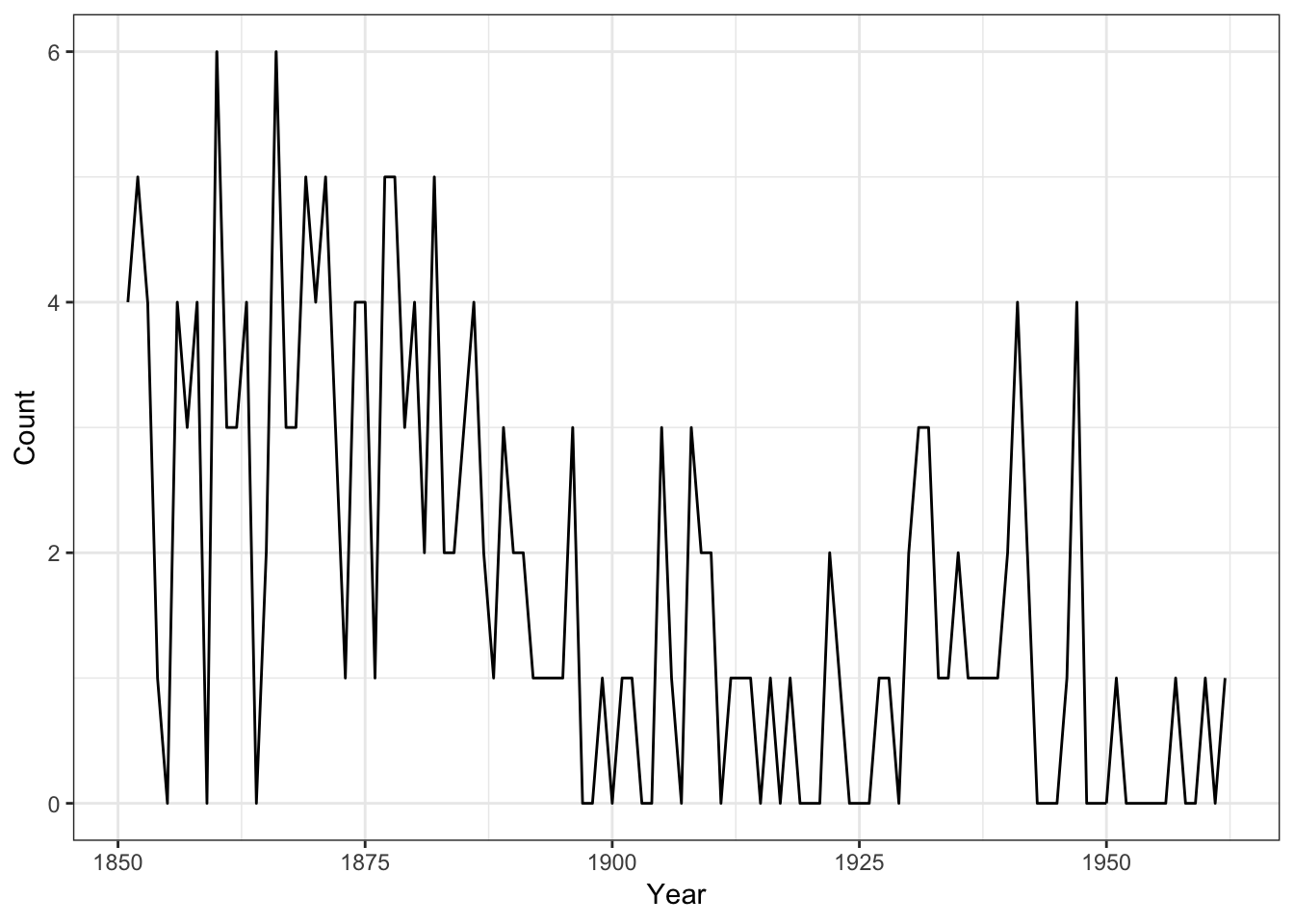
It suggests that the rate of accidents decreased sometime around 1900.
So let us define the statistical model that may fit to the data and let us give a Bayesian estimation of the parameters.
Let us denote by \(\tau\) the change-point time and let us assume that before \(\tau\) the number of disasters follows a Poisson distribution with parameter \(\lambda_1\) and it follows after \(\tau\) also a Poisson distribution with parameter \(\lambda_2\). We will expect then to have \(\lambda_2< \lambda_1\). We may consider later more than one changepoint.
We will first assume a non-informative prior distribution on the vector of parameters \(\theta=(\lambda_1,\lambda_2,\tau)\): \[\pi(\lambda_1,\lambda_2,\tau)\propto \mathbb{1}_{\mathbb{R}^2}(\lambda_1,\lambda_2)\times\mathbb{1}_{\{1,\ldots,N\}}(\tau)\] where \(N\) is the number of years of the study.
Hence the BUGS code of the model is:
Let us notice that this version uses a slightly different parametrization, with the first element of b as \(\log(\lambda_1)\) and the second as \(\log(\lambda_2)-\log(\lambda_1)\).
The R implementation
We will run the BUGS code using OpenBUGS and the R package R2OpenBUGS:
sink('exChangePointPoiss.txt')
cat("
model {
      for (year in 1:N) {
           D[year] ~ dpois(mu[year])
           log(mu[year]) <- b[1] + step(year - changeyear) * b[2]
      }
      for (j in 1:2) { b[j] ~ dnorm(0.0, 1.0E-6) }
      changeyear ~ dunif(1,N)
    }
",fill=T)
sink()

## Data
dt<-list(D<-CoalDisast$Count,N=nrow(CoalDisast))

## Initials
inits=function(){
  inits=list(b=rnorm(2),changeyear=sample(size = 1,x = 1:nrow(CoalDisast)))
}

## Params
params<-c("b","changeyear")

## Running the MC
library(R2OpenBUGS)
filename<-'exChangePointPoiss.txt'
outCPPoiss <-bugs(dt,inits,params,filename,codaPkg=F,
                n.thin =1, n.iter=10000,debug=F,
                n.chains = 3,working.directory=getwd())
outCPPoiss
Or if you work with MAC OS.
OpenBUGS.pgm="/Users/dhafermalouche/.wine/drive_c/Program Files (x86)/OpenBUGS/OpenBUGS323/OpenBUGS.exe"
outCPPoiss <-bugs(dt,inits,params,filename,codaPkg=F,
                n.thin =1, n.iter=10000,debug=F,
                n.chains = 3,working.directory=getwd(),
                OpenBUGS.pgm=OpenBUGS.pgm, useWINE=T)
## Inference for Bugs model at "exChangePointPoiss.txt",
## Current: 3 chains, each with 10000 iterations (first 5000 discarded)
## Cumulative: n.sims = 15000 iterations saved
## mean sd 2.5% 25% 50% 75% 97.5% Rhat n.eff
## b[1] 1.1 0.1 0.9 1.1 1.1 1.2 1.3 1 15000
## b[2] -1.2 0.2 -1.5 -1.3 -1.2 -1.1 -0.9 1 15000
## changeyear 40.5 2.5 36.1 39.1 40.7 41.8 46.4 1 15000
## deviance 341.2 2.6 337.9 339.3 340.6 342.4 347.9 1 12000
##
## For each parameter, n.eff is a crude measure of effective sample size,
## and Rhat is the potential scale reduction factor (at convergence, Rhat=1).
##
## DIC info (using the rule, pD = Dbar-Dhat)
## pD = 3.0 and DIC = 344.2
## DIC is an estimate of expected predictive error (lower deviance is better).Let us make a diagnostic of the convergence of the Markov Chains:
- Trace of the MC
> dim(outCPPoiss$sims.array)## [1] 5000 3 4> library(coda)
> b1=mcmc(outCPPoiss$sims.array[,,1])
> dim(b1)## [1] 5000 3> matplot(b1,col=c("red","green","blue"),type="l",ylab=expression(b_1))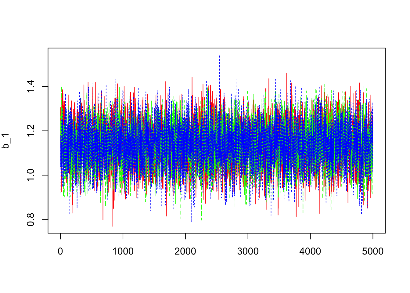
> b2=mcmc(outCPPoiss$sims.array[,,2])
> dim(b2)
## [1] 5000 3> matplot(b2,col=c("red","green","blue"),type="l",ylab=expression(b_2))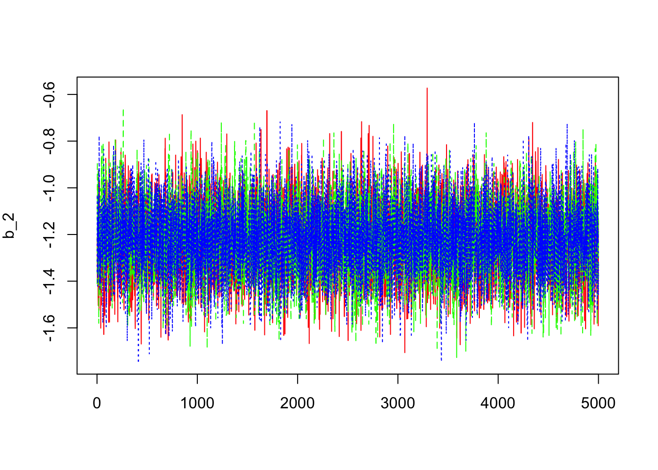
> changeyear=mcmc(outCPPoiss$sims.array[,,3])
> dim(changeyear)
## [1] 5000 3> matplot(changeyear,col=c("red","green","blue"),type="l",ylab="changeyear")
- \(\widehat{R}\) or Gelman diagnostics
> gelman.diag(list(b1[,1],b1[,2],b1[,3]))## Potential scale reduction factors:
##
## Point est. Upper C.I.
## [1,] 1 1> gelman.plot(list(changeyear[,1],changeyear[,2],changeyear[,3]))
> gelman.diag(list(changeyear[,1],changeyear[,2],changeyear[,3]))## Potential scale reduction factors:
##
## Point est. Upper C.I.
## [1,] 1 1> gelman.plot(list(changeyear[,1],changeyear[,2],changeyear[,3]))
> gelman.diag(list(changeyear[,1],changeyear[,2],changeyear[,3]))## Potential scale reduction factors:
##
## Point est. Upper C.I.
## [1,] 1 1> gelman.plot(list(b1[,1],b1[,2],b1[,3]))
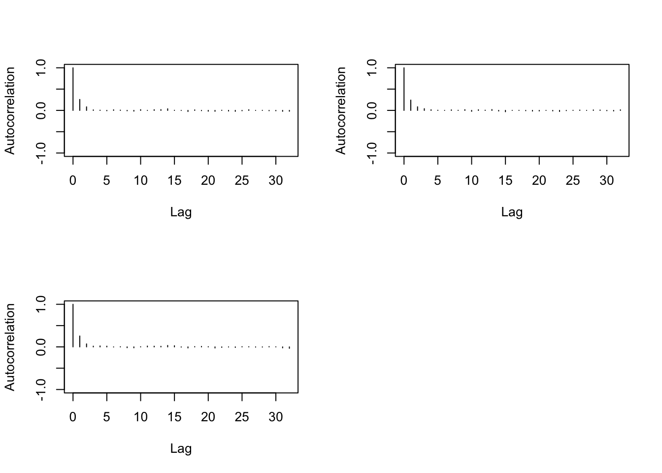
- Autocorrelation
> autocorr.diag(b1)## [,1] [,2] [,3]
## Lag 0 1.000000000 1.000000000 1.000000000
## Lag 1 0.257092833 0.242148271 0.255831639
## Lag 5 -0.007711446 0.003761342 0.017163560
## Lag 10 0.017128683 -0.021708080 0.003541084
## Lag 50 0.010435906 0.007931565 -0.018354853> autocorr.plot(b1)