Visualization with ggpubr package
We will show in this note how to use ggpubr package to draw nice boxplots, violin and density plots. We will be using as an Example genetic data such the TCGA data. It’s a dataset known as the Cancer Genome Atlas (TCGA) data is a publicly available data containing clinical and genomic data across 33 cancer types. It’s a set of several data that include gene expression, CNV profiling, SNP genotyping, DNA methylation, miRNA profiling, exome sequencing, and other types of data. This data is then available in the R package RTCGA build by Marcin Kosinski and Przemyslaw Biecek. Here’s a link where you can find instructions on how you can install the package and use the data: https://bioconductor.org/packages/release/bioc/html/RTCGA.html
Getting the TCGA data
The following R code installs the core RTCGA package as well as the clinical and mRNA gene expression data packages.
- Load the bioconductor installer.
> source("https://bioconductor.org/biocLite.R")
> biocLite("RTCGA")- Install the main RTCGA package
> library(RTCGA)
> installTCGA("RTCGA.mRNA")
> library(RTCGA.mRNA) # Run this on R not in RStudio
> library(RTCGA)## Welcome to the RTCGA (version: 1.12.0).> load("data_mRNA.RData")Here’s then the dataset. Each cell is a data.frame and it represents the number of obs.
> infoTCGA() ## Cohort BCR Clinical CN LowP Methylation mRNA mRNASeq
## ACC-counts ACC 92 92 90 0 80 0 79
## BLCA-counts BLCA 412 412 410 112 412 0 408
## BRCA-counts BRCA 1098 1097 1089 19 1097 526 1093
## CESC-counts CESC 307 307 295 50 307 0 304
## CHOL-counts CHOL 51 45 36 0 36 0 36
## COAD-counts COAD 460 458 451 69 457 153 457
## COADREAD-counts COADREAD 631 629 616 104 622 222 623
## DLBC-counts DLBC 58 48 48 0 48 0 48
## ESCA-counts ESCA 185 185 184 51 185 0 184
## FPPP-counts FPPP 38 38 0 0 0 0 0
## GBM-counts GBM 613 595 577 0 420 540 160
## GBMLGG-counts GBMLGG 1129 1110 1090 52 936 567 676
## HNSC-counts HNSC 528 528 522 108 528 0 520
## KICH-counts KICH 113 113 66 0 66 0 66
## KIPAN-counts KIPAN 973 941 883 0 892 88 889
## KIRC-counts KIRC 537 537 528 0 535 72 533
## KIRP-counts KIRP 323 291 289 0 291 16 290
## LAML-counts LAML 200 200 197 0 194 0 179
## LGG-counts LGG 516 515 513 52 516 27 516
## LIHC-counts LIHC 377 377 370 0 377 0 371
## LUAD-counts LUAD 585 522 516 120 578 32 515
## LUSC-counts LUSC 504 504 501 0 503 154 501
## MESO-counts MESO 87 87 87 0 87 0 87
## OV-counts OV 602 591 586 0 594 574 304
## PAAD-counts PAAD 185 185 184 0 184 0 178
## PCPG-counts PCPG 179 179 175 0 179 0 179
## PRAD-counts PRAD 499 499 492 115 498 0 497
## READ-counts READ 171 171 165 35 165 69 166
## SARC-counts SARC 261 261 257 0 261 0 259
## SKCM-counts SKCM 470 470 469 118 470 0 469
## STAD-counts STAD 443 443 442 107 443 0 415
## STES-counts STES 628 628 626 158 628 0 599
## TGCT-counts TGCT 150 134 150 0 150 0 150
## THCA-counts THCA 503 503 499 98 503 0 501
## THYM-counts THYM 124 124 123 0 124 0 120
## UCEC-counts UCEC 560 548 540 106 547 54 545
## UCS-counts UCS 57 57 56 0 57 0 57
## UVM-counts UVM 80 80 80 51 80 0 80
## miR miRSeq RPPA MAF rawMAF
## ACC-counts 0 80 46 90 0
## BLCA-counts 0 409 344 130 395
## BRCA-counts 0 1078 887 977 0
## CESC-counts 0 307 173 194 0
## CHOL-counts 0 36 30 35 0
## COAD-counts 0 406 360 154 367
## COADREAD-counts 0 549 491 223 489
## DLBC-counts 0 47 33 48 0
## ESCA-counts 0 184 126 185 0
## FPPP-counts 0 23 0 0 0
## GBM-counts 565 0 238 290 290
## GBMLGG-counts 565 512 668 576 806
## HNSC-counts 0 523 212 279 510
## KICH-counts 0 66 63 66 66
## KIPAN-counts 0 873 756 644 799
## KIRC-counts 0 516 478 417 451
## KIRP-counts 0 291 215 161 282
## LAML-counts 0 188 0 197 0
## LGG-counts 0 512 430 286 516
## LIHC-counts 0 372 63 198 373
## LUAD-counts 0 513 365 230 542
## LUSC-counts 0 478 328 178 0
## MESO-counts 0 87 63 0 0
## OV-counts 570 453 426 316 469
## PAAD-counts 0 178 123 150 184
## PCPG-counts 0 179 80 179 0
## PRAD-counts 0 494 352 332 498
## READ-counts 0 143 131 69 122
## SARC-counts 0 259 223 247 0
## SKCM-counts 0 448 353 343 366
## STAD-counts 0 436 357 289 395
## STES-counts 0 620 483 474 395
## TGCT-counts 0 150 118 149 0
## THCA-counts 0 502 222 402 496
## THYM-counts 0 124 90 123 0
## UCEC-counts 0 538 440 248 0
## UCS-counts 0 56 48 57 0
## UVM-counts 0 80 12 80 0We will now extract the mRNA expression for five genes of interest
- GATA3, PTEN, XBP1, ESR1 and MUC1
from 3 different data sets:
- Breast invasive carcinoma (BRCA),
- Ovarian serous cystadenocarcinoma (OV) and
- Lung squamous cell carcinoma (LUSC)
and we will merge them in the same dataset
> expr <- expressionsTCGA(BRCA.mRNA, OV.mRNA, LUSC.mRNA,
+                         extract.cols = c("GATA3",
+                                          "PTEN", "XBP1",
+                                          "ESR1", "MUC1"))
The new data has the following characteristics
> dim(expr)## [1] 1305 7> colnames(expr)## [1] "bcr_patient_barcode" "dataset" "GATA3"
## [4] "PTEN" "XBP1" "ESR1"
## [7] "MUC1"> head(expr)## # A tibble: 6 x 7
## bcr_patient_barcode dataset GATA3 PTEN XBP1 ESR1 MUC1
## <chr> <chr> <dbl> <dbl> <dbl> <dbl> <dbl>
## 1 TCGA-A1-A0SD-01A-11R-A115-07 BRCA.mRNA 2.87 1.36 2.98 3.08 1.65
## 2 TCGA-A1-A0SE-01A-11R-A084-07 BRCA.mRNA 2.17 0.428 2.55 2.39 3.08
## 3 TCGA-A1-A0SH-01A-11R-A084-07 BRCA.mRNA 1.32 1.31 3.02 0.791 2.99
## 4 TCGA-A1-A0SJ-01A-11R-A084-07 BRCA.mRNA 1.84 0.810 3.13 2.50 -1.92
## 5 TCGA-A1-A0SK-01A-12R-A084-07 BRCA.mRNA -6.03 0.251 -1.45 -4.86 -1.17
## 6 TCGA-A1-A0SM-01A-11R-A084-07 BRCA.mRNA 1.80 1.31 4.04 2.80 3.53Let’s display the number of sample in each data set:
> nb_samples <- table(expr$dataset)
> nb_samples
##
## BRCA.mRNA LUSC.mRNA OV.mRNA
## 590 154 561We simplify data set names by removing the “mRNA” tag.
> expr$dataset <- gsub(pattern = ".mRNA",
+                      replacement = "",  expr$dataset)
We simplify also the patients’ barcode column. The following R code will change the barcodes into BRCA1, BRCA2, …, OV1, OV2, …., etc
> expr$bcr_patient_barcode <- paste0(expr$dataset,
+                                    c(1:590, 1:561, 1:154))
Finaly our dataset looks like the following
> expr## # A tibble: 1,305 x 7
## bcr_patient_barcode dataset GATA3 PTEN XBP1 ESR1 MUC1
## <chr> <chr> <dbl> <dbl> <dbl> <dbl> <dbl>
## 1 BRCA1 BRCA 2.87 1.36 2.98 3.08 1.65
## 2 BRCA2 BRCA 2.17 0.428 2.55 2.39 3.08
## 3 BRCA3 BRCA 1.32 1.31 3.02 0.791 2.99
## 4 BRCA4 BRCA 1.84 0.810 3.13 2.50 -1.92
## 5 BRCA5 BRCA -6.03 0.251 -1.45 -4.86 -1.17
## 6 BRCA6 BRCA 1.80 1.31 4.04 2.80 3.53
## 7 BRCA7 BRCA -4.88 -0.237 -0.725 -4.49 -1.46
## 8 BRCA8 BRCA -3.14 -1.24 -1.19 -1.63 -0.987
## 9 BRCA9 BRCA 2.03 1.21 2.28 4.12 0.668
## 10 BRCA10 BRCA -0.293 0.288 -1.61 0.473 0.0115
## # ... with 1,295 more rowsBoxplots
Installing ggpubr package
Let’s first install ggpubr from kassambra Github account
> if(!require(devtools)) install.packages("devtools")
> devtools::install_github("kassambara/ggpubr")
Let’s now load ggpubr in R
> library(ggpubr)## Loading required package: ggplot2## Loading required package: magrittrFirst boxplot
I will know show how to create a box plot of a gene expression profile, colored by groups (here dataset/cancer type). We show the level of expression of the gene GATA3 accorrding to each data sample.
> ggboxplot(expr, x = "dataset", y = "GATA3",
+           title = "GATA3", ylab = "Expression",
+           color = "dataset", palette = "jco")
Same thing with the PTEN gene:
> ggboxplot(expr, x = "dataset", y = "PTEN",
+           title = "PTEN", ylab = "Expression",
+           color = "dataset", palette = "jco")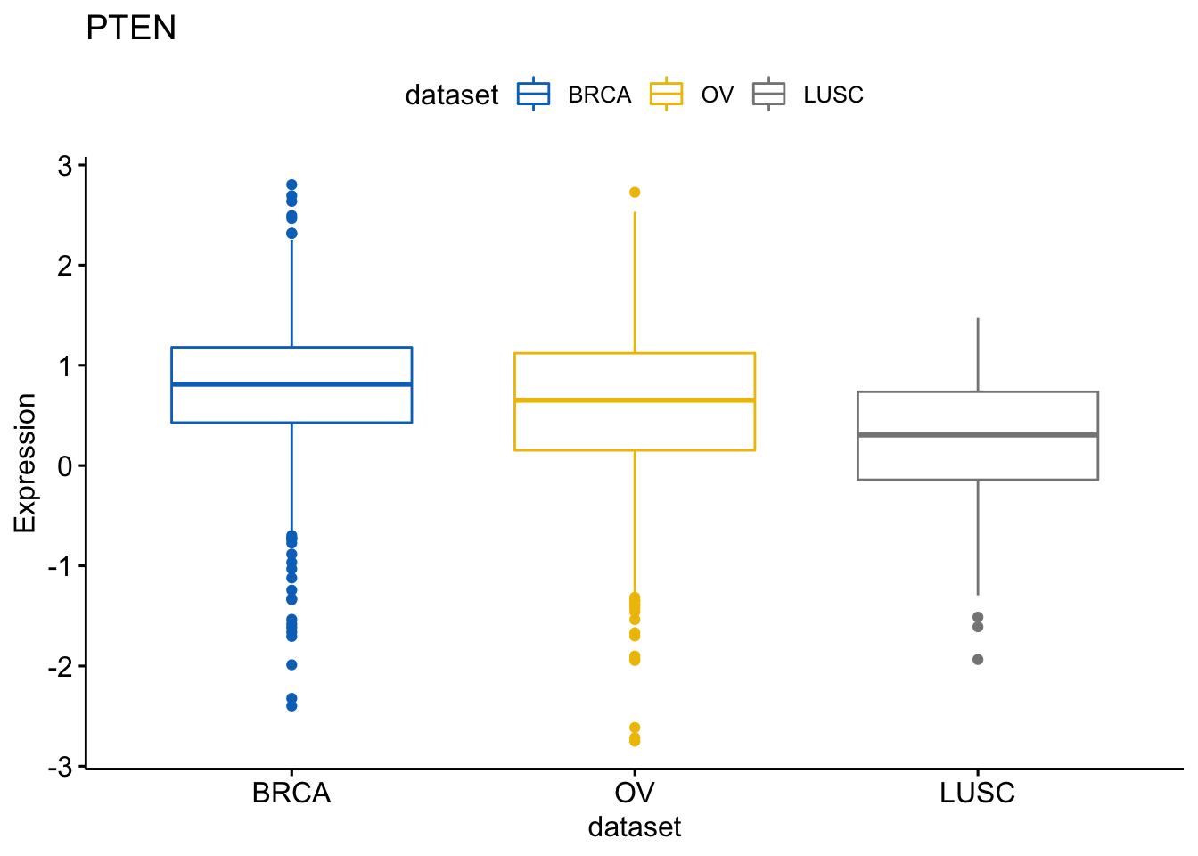
Know we create a list of boxplots
> p <- ggboxplot(expr, x = "dataset",
+                y = c("GATA3", "PTEN", "XBP1"),
+                title = c("GATA3", "PTEN", "XBP1"),
+                 ylab = "Expression",
+                color = "dataset", palette = "jco")
We can view the boxplot according the Gene GATA3
> p$GATA3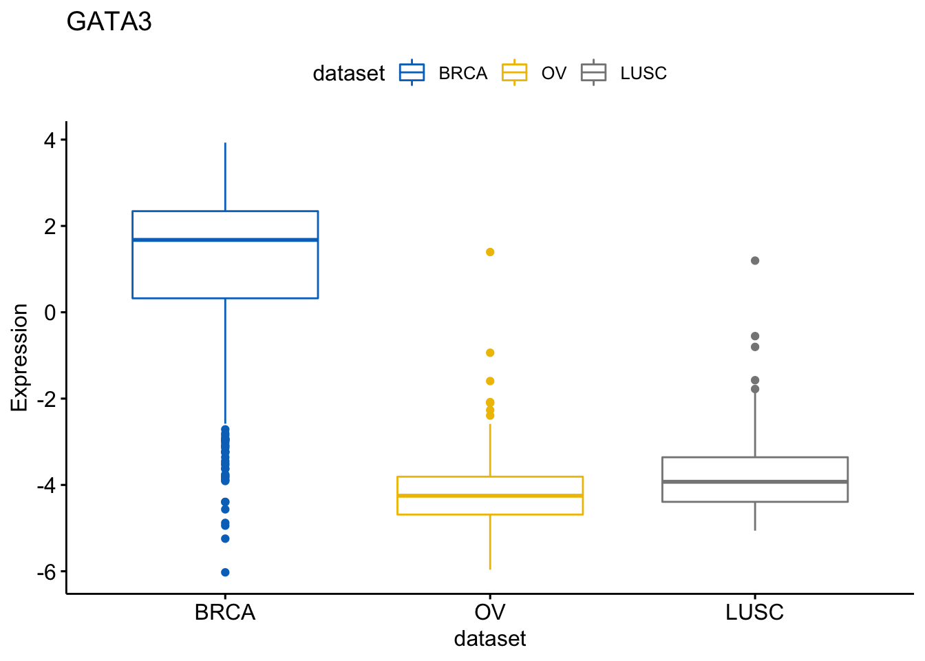
and the gene PTEN
> p$PTEN
and the gene XBP1
> p$XBP1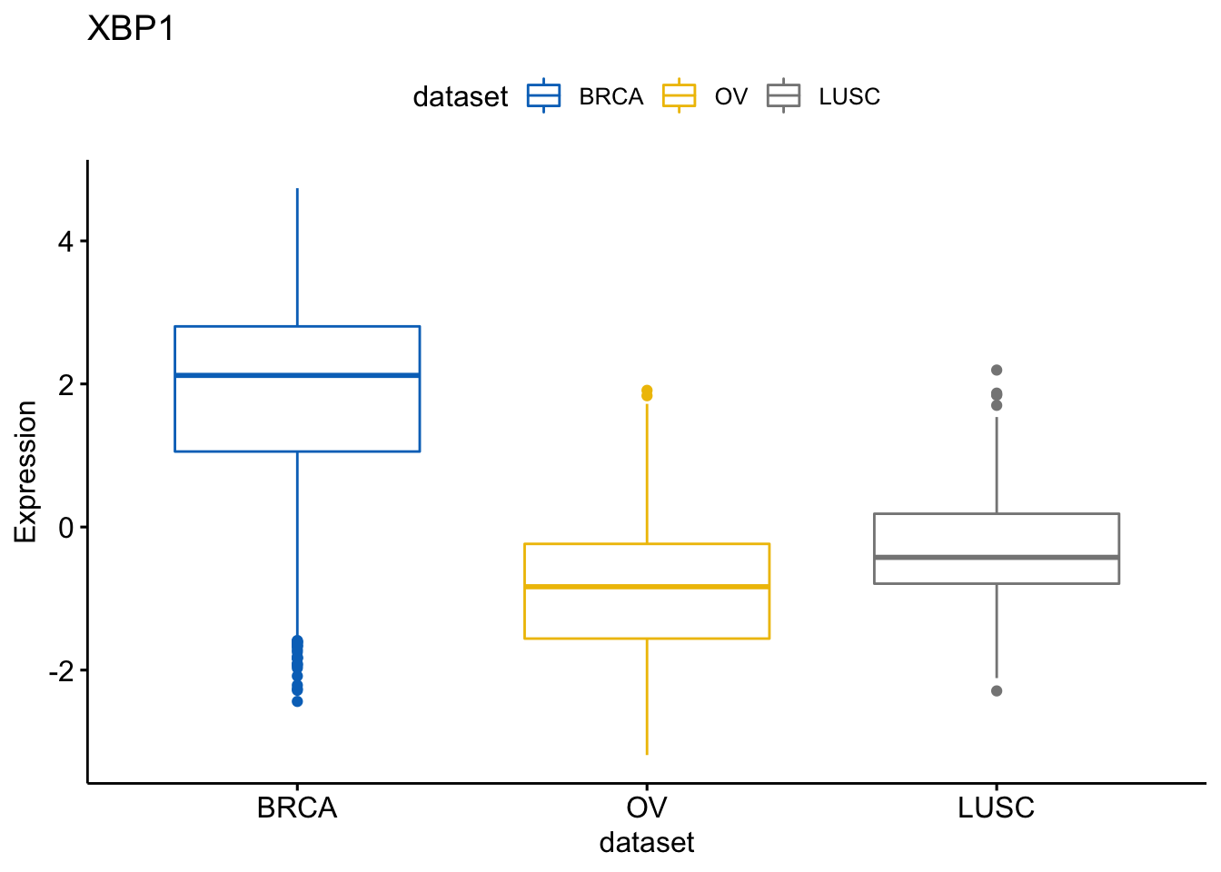
Pairwise comparison
Now we would like to compare the means and perform the an ANOVA. We will then ask to add the p-values of the pairwise comparison
> my_comparisons <- list(c("BRCA", "OV"), c("OV", "LUSC"))
> ggboxplot(expr, x = "dataset", y = "GATA3",
+           title = "GATA3", ylab = "Expression",
+           color = "dataset", palette = "jco")+
+   stat_compare_means(comparisons = my_comparisons)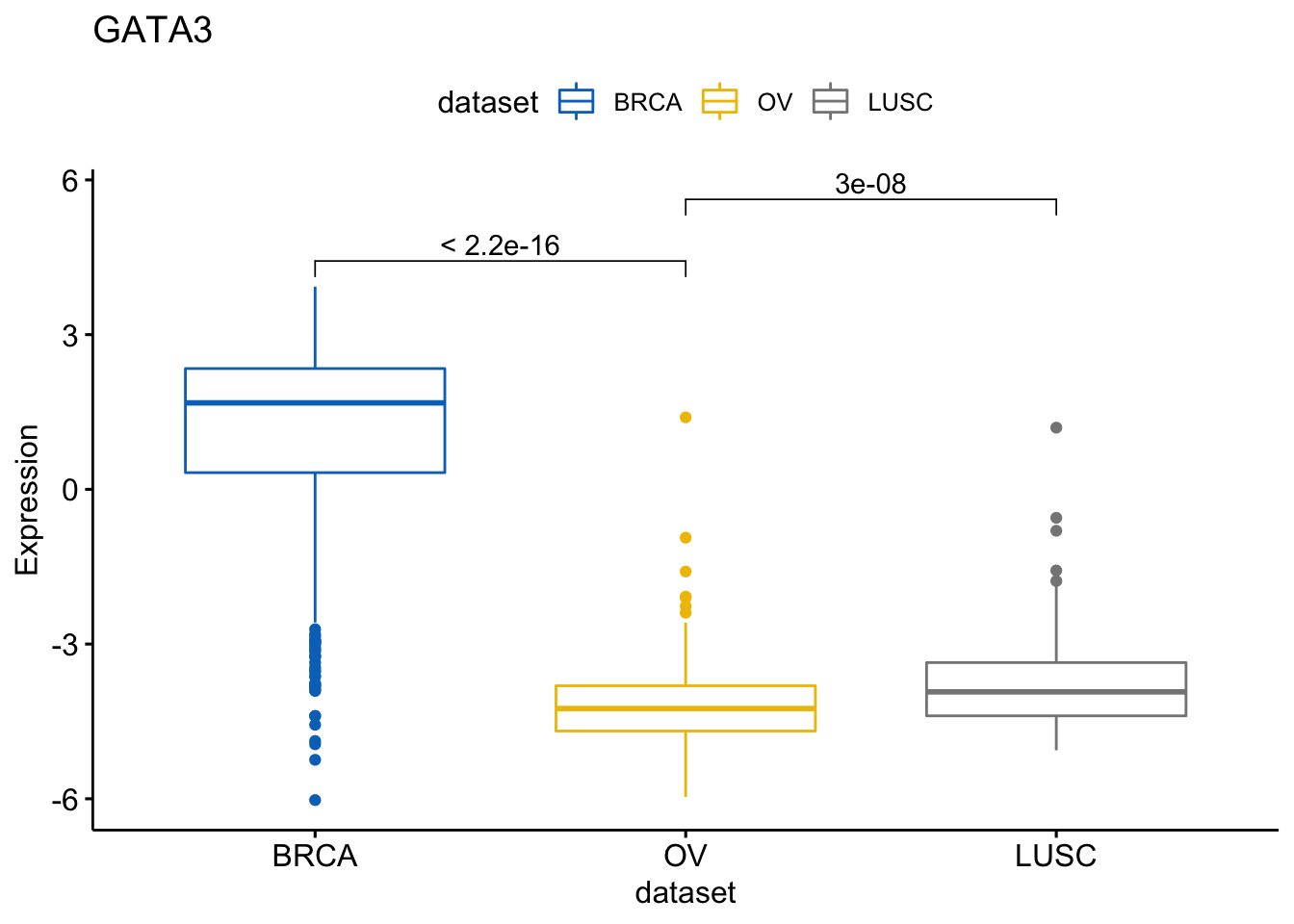
We can then with the same method show more comparisons
> my_comparisons <- list(c("BRCA", "OV"),
+                        c("OV", "LUSC"),
+                        c("BRCA","LUSC"))
> ggboxplot(expr, x = "dataset", y = "GATA3",
+           title = "GATA3", ylab = "Expression",
+           color = "dataset", palette = "jco")+
+   stat_compare_means(comparisons = my_comparisons)
We can also compare mean between many genes at the same time:
> comp_data=compare_means(c(GATA3, PTEN, XBP1) ~ dataset, data = expr)
> comp_data
## # A tibble: 9 x 8
## .y. group1 group2 p p.adj p.format p.signif method
## <fct> <chr> <chr> <dbl> <dbl> <chr> <chr> <chr>
## 1 GATA3 BRCA OV 1.11e-177 3.30e-177 < 2e-16 **** Wilcoxon
## 2 GATA3 BRCA LUSC 6.68e- 73 1.30e- 72 < 2e-16 **** Wilcoxon
## 3 GATA3 OV LUSC 2.97e- 8 3.00e- 8 3.0e-08 **** Wilcoxon
## 4 PTEN BRCA OV 6.79e- 5 6.80e- 5 6.8e-05 **** Wilcoxon
## 5 PTEN BRCA LUSC 1.04e- 16 3.10e- 16 < 2e-16 **** Wilcoxon
## 6 PTEN OV LUSC 1.28e- 7 2.60e- 7 1.3e-07 **** Wilcoxon
## 7 XBP1 BRCA OV 2.55e-123 7.70e-123 < 2e-16 **** Wilcoxon
## 8 XBP1 BRCA LUSC 1.95e- 42 3.90e- 42 < 2e-16 **** Wilcoxon
## 9 XBP1 OV LUSC 4.24e- 11 4.20e- 11 4.2e-11 **** WilcoxonBoxplot manipulations
You can then select items (here cancer types) to display.
> ggboxplot(expr, x = "dataset", y = "GATA3",
+           title = "GATA3", ylab = "Expression",
+           color = "dataset", palette = "jco",
+           select = c("BRCA", "OV"))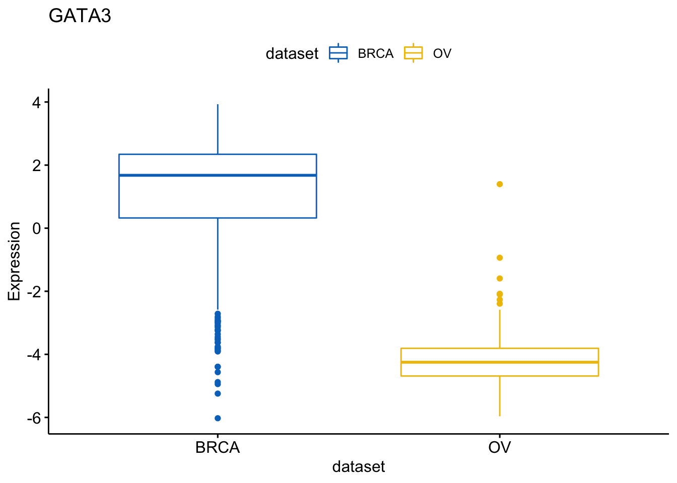
You can also remove items (here cancer types).
> ggboxplot(expr, x = "dataset", y = "GATA3",
+           title = "GATA3", ylab = "Expression",
+           color = "dataset", palette = "jco",
+           remove = "BRCA")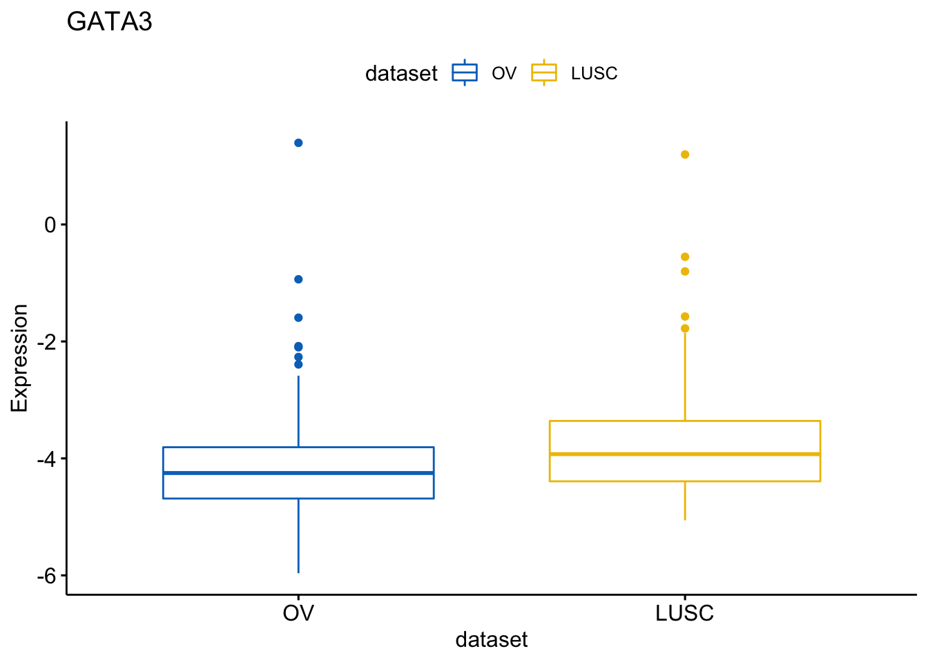
It’s also possible to change the order of the dataset on x axis
> ggboxplot(expr, x = "dataset", y = "GATA3",
+           title = "GATA3", ylab = "Expression",
+           color = "dataset", palette = "jco",
+           order = c("LUSC", "OV", "BRCA"))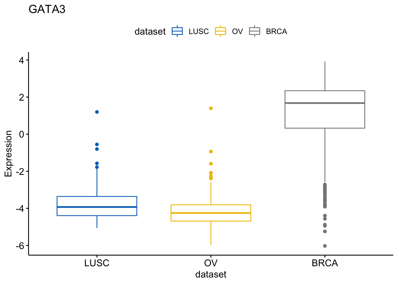
We can also create horizontal plots
> ggboxplot(expr, x = "dataset", y = "GATA3",
+           title = "GATA3", ylab = "Expression",
+           color = "dataset", palette = "jco",
+           rotate = TRUE)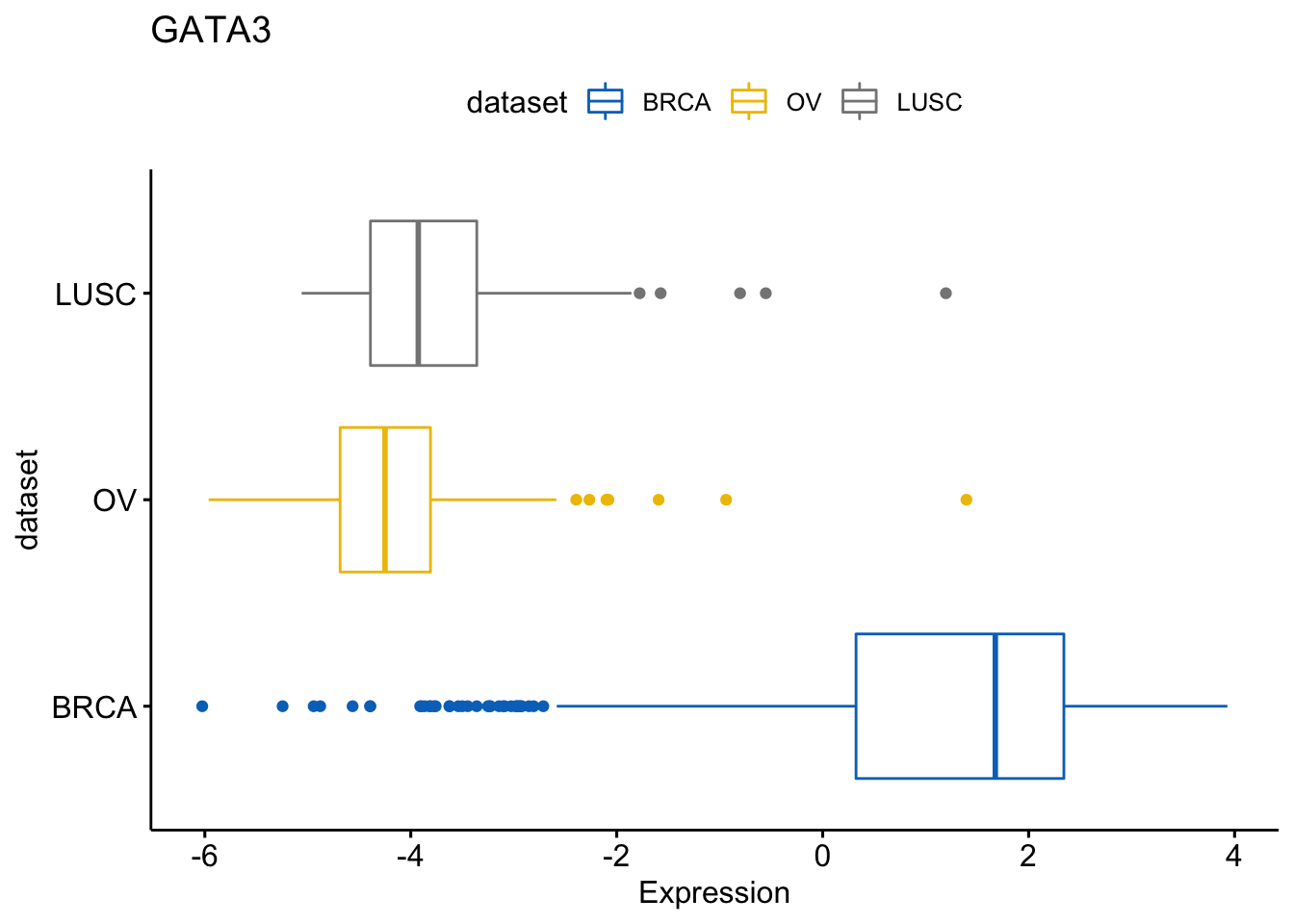
It’s also possible to combine the three gene expression plots into a multi-panel plot, use the argument combine = TRUE:
> ggboxplot(expr, x = "dataset",
+           y = c("GATA3", "PTEN", "XBP1"),
+           combine = TRUE,
+           ylab = "Expression",
+           color = "dataset", palette = "jco")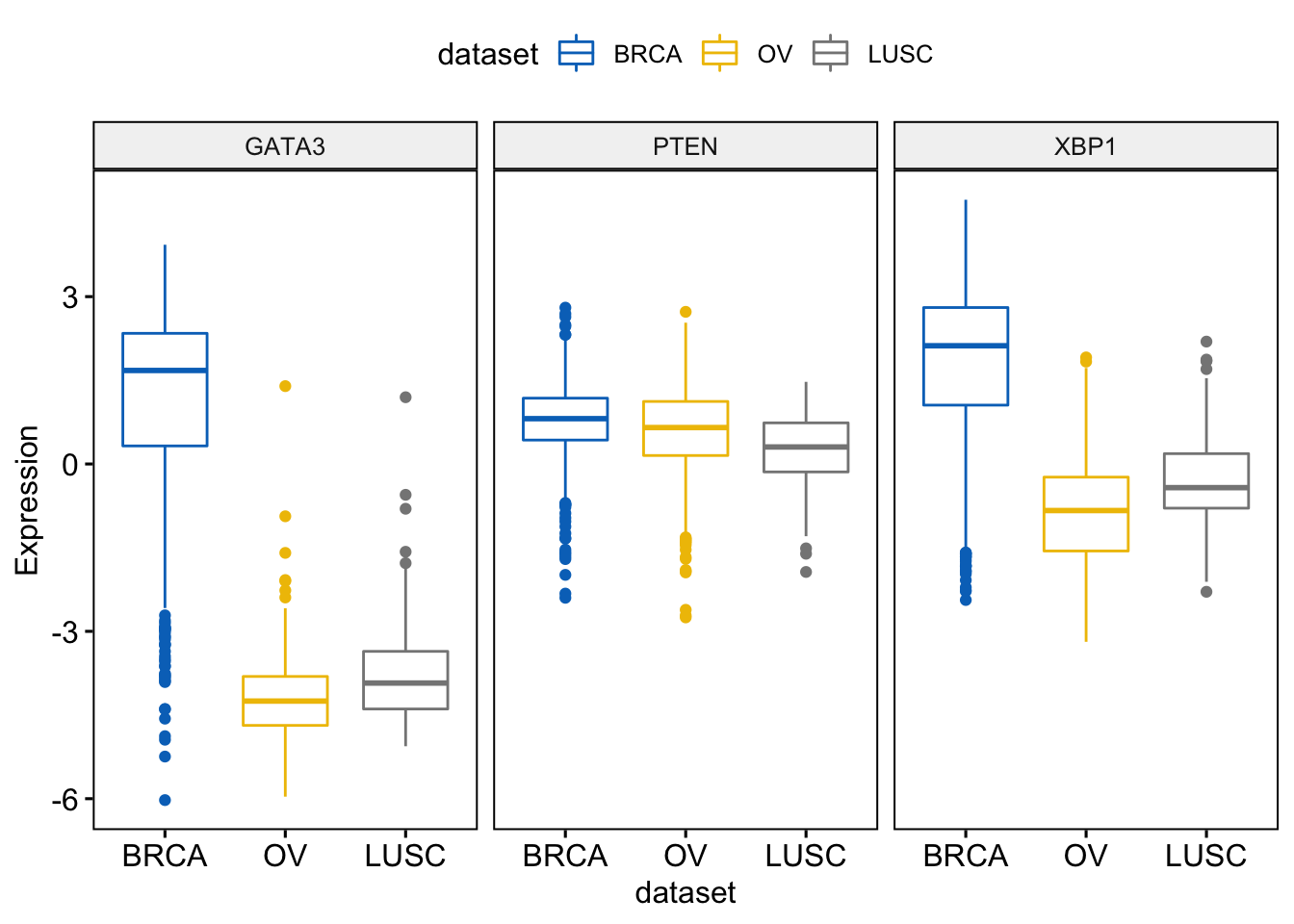
We can merge the 3 plots using the argument merge = TRUE:
> ggboxplot(expr, x = "dataset",
+           y = c("GATA3", "PTEN", "XBP1"),
+           merge = TRUE,
+           ylab = "Expression",
+           palette = "jco")
We can merge the 3 plots using the argument merge = "asis":
> ggboxplot(expr, x = "dataset",
+           y = c("GATA3", "PTEN", "XBP1"),
+           merge = "asis",
+           ylab = "Expression",
+           palette = "jco")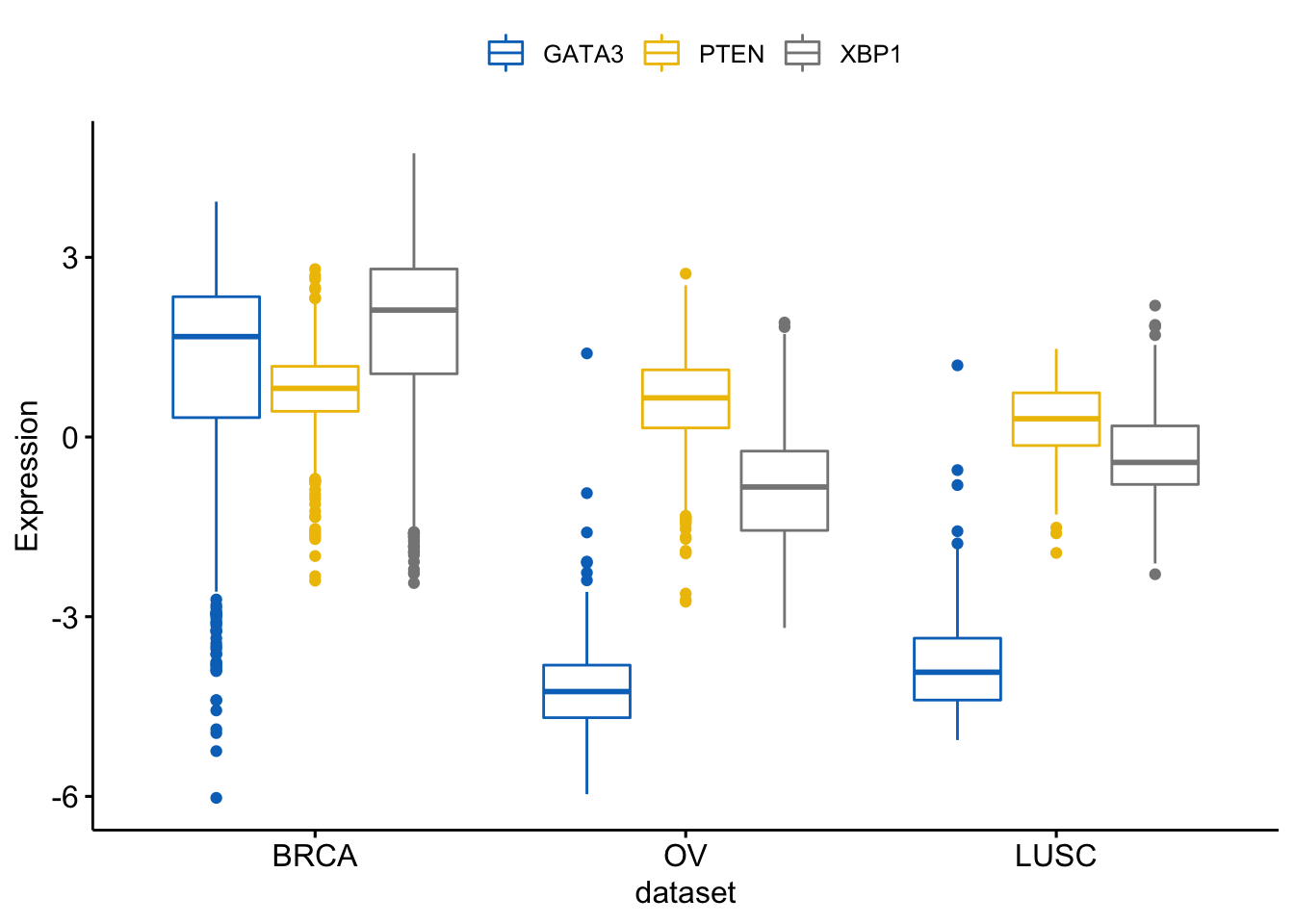
The y variables (i.e.: genes) become x tick labels and the x variable (i.e.: dataset) becomes the grouping variable. To do this, use the argument merge = “flip”:
> ggboxplot(expr, x = "dataset",
+           y = c("GATA3", "PTEN", "XBP1"),
+           merge = "flip",
+           ylab = "Expression",
+           palette = "jco")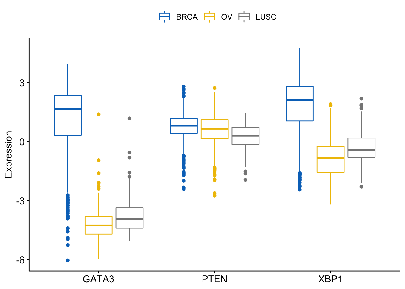
Adding decorations
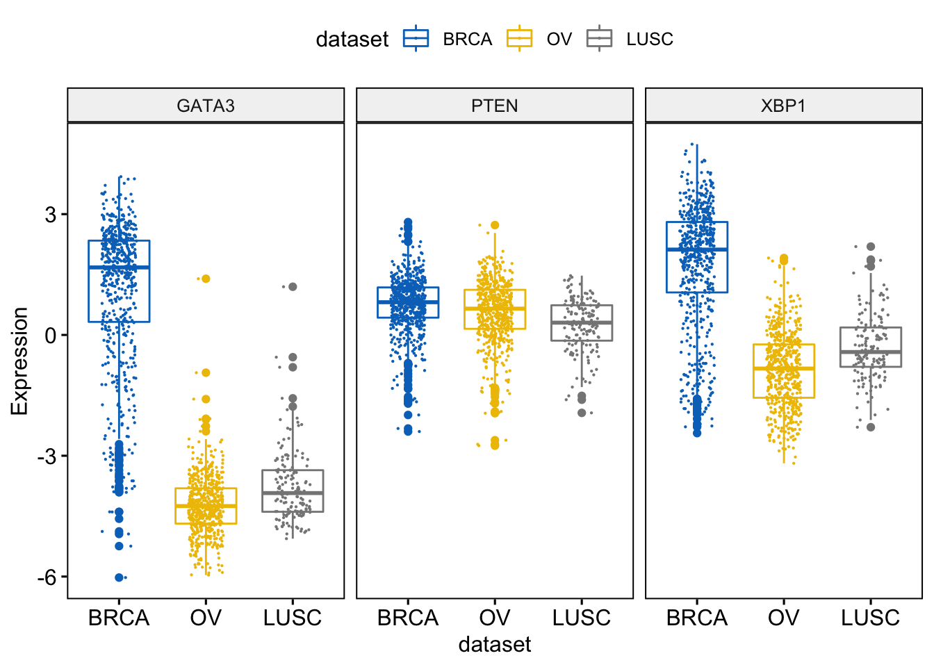
We will add jittered points on the boxplot.
> ggboxplot(expr, x = "dataset",
+           y = c("GATA3", "PTEN", "XBP1"),
+           combine = TRUE,
+           color = "dataset", palette = "jco",
+           ylab = "Expression",
+           add = "jitter",                              # Add jittered points
+           add.params = list(size = 0.1, jitter = 0.2)  # Point size and the amount of jittering
+ )
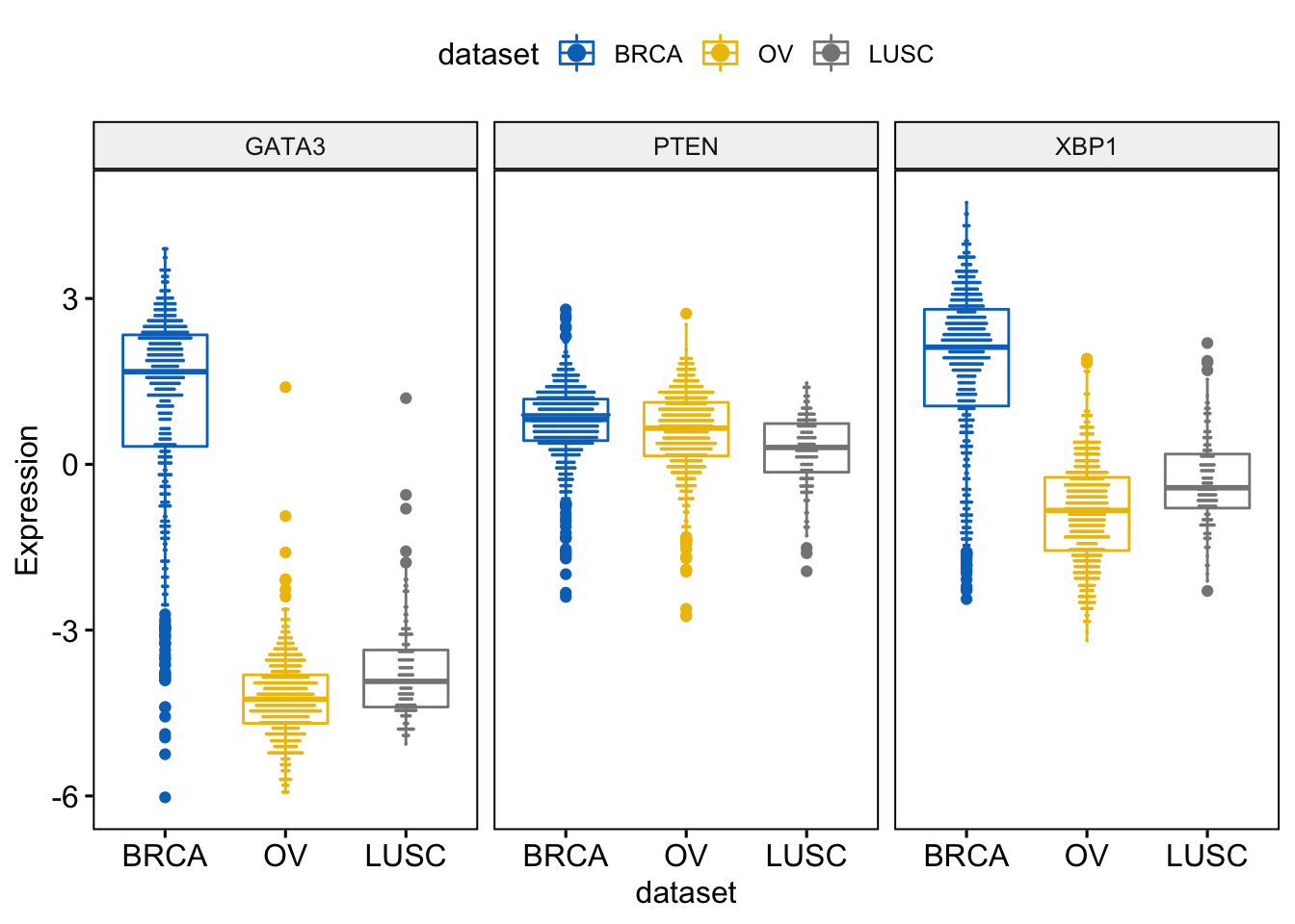
We can also add and adjust a dotplot.
> ggboxplot(expr, x = "dataset",
+             y = c("GATA3", "PTEN", "XBP1"),
+             combine = TRUE,
+             color = "dataset", palette = "jco",
+             ylab = "Expression",
+             add = "dotplot",                              # Add dotplot
+             add.params = list(binwidth = 0.1, dotsize = 0.3)
+   )
We can label the boxplot by showing the names of the samples with the top \(n\) highest or lowest values.
You can use the following arguments:
label: the name of the column containing point labels.label.select: can be of two formats:- a character vector specifying some labels to show.
- a list containing one or the combination of the following components:
top.upandtop.down: to display the labels of the top up/down points.
Example,
label.select = list(top.up = 10, top.down = 4) or
label.select = list(criteria = “y > 3.9 & y < 5 & x %in% c(‘BRCA’, ‘OV’)”)
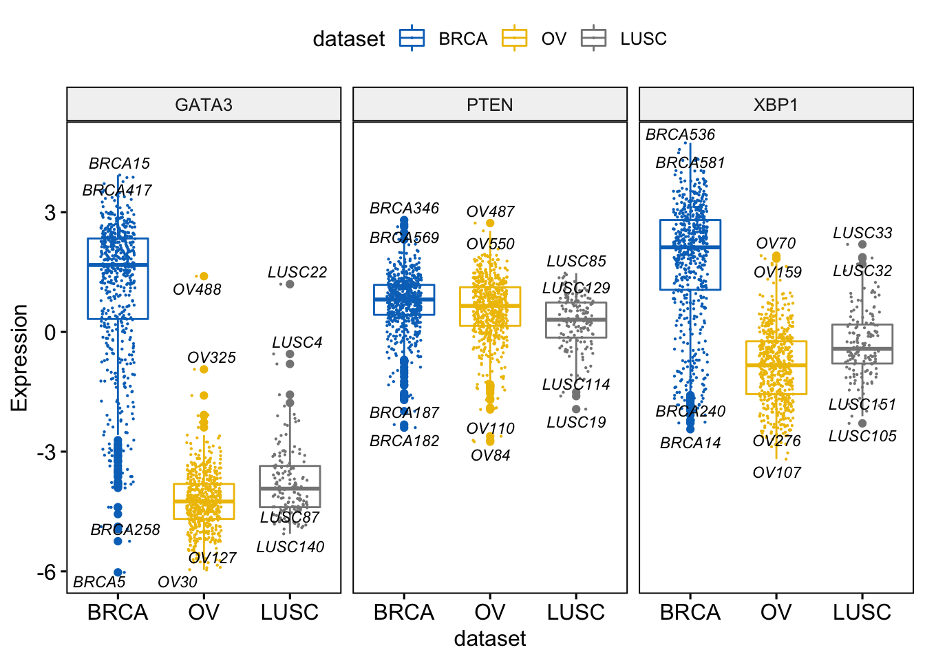
> ggboxplot(expr, x = "dataset",
+             y = c("GATA3", "PTEN", "XBP1"),
+             combine = TRUE,
+             color = "dataset", palette = "jco",
+             ylab = "Expression",
+             add = "jitter",                               # Add jittered points
+             add.params = list(size = 0.1, jitter = 0.2),  # Point size and the amount of jittering
+             label = "bcr_patient_barcode",                # column containing point labels
+             label.select = list(top.up = 2, top.down = 2),# Select some labels to display
+             font.label = list(size = 9, face = "italic"), # label font
+             repel = TRUE                                  # Avoid label text overplotting
+   )
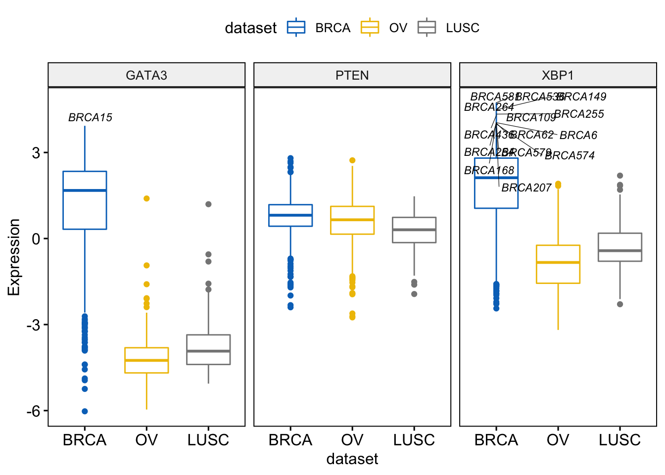
> label.select.criteria <- list(criteria = "`y` > 3.9 & `x` %in% c('BRCA', 'OV')")
>   ggboxplot(expr, x = "dataset",
+             y = c("GATA3", "PTEN", "XBP1"),
+             combine = TRUE,
+             color = "dataset", palette = "jco",
+             ylab = "Expression",
+             label = "bcr_patient_barcode",              # column containing point labels
+             label.select = label.select.criteria,       # Select some labels to display
+             font.label = list(size = 9, face = "italic"), # label font
+             repel = TRUE                                # Avoid label text overplotting
+   )
Violin plots

Violin + Boxplot
>  ggviolin(expr, x = "dataset",
+            y = c("GATA3", "PTEN", "XBP1"),
+            combine = TRUE,
+            color = "dataset", palette = "jco",
+            ylab = "Expression",
+            add = "boxplot")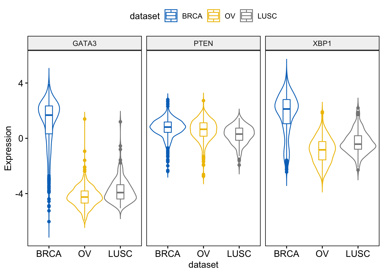
Displaying the descriptive statistics
> library(reshape)
> dt=as.data.frame(expr[,-1])
> expr2=melt(dt)
## Using dataset as id variables> head(expr2,2)## dataset variable value
## 1 BRCA GATA3 2.87050
## 2 BRCA GATA3 2.16625> res<-desc_statby(expr2,measure.var = "value",grps=c("dataset","variable"))
> res## dataset variable length min max median mean
## 1 BRCA GATA3 590 -6.025250 3.930000 1.6763750 1.1035732
## 2 BRCA PTEN 590 -2.398357 2.802786 0.8123929 0.7486928
## 3 BRCA XBP1 590 -2.438250 4.736750 2.1194167 1.7498139
## 4 BRCA ESR1 590 -4.860667 6.110833 3.0645833 2.2982359
## 5 BRCA MUC1 590 -2.793875 4.280500 2.2476875 1.8527130
## 6 LUSC GATA3 154 -5.059500 1.196625 -3.9270625 -3.7584818
## 7 LUSC PTEN 154 -1.935429 1.472357 0.3048571 0.2516035
## 8 LUSC XBP1 154 -2.291083 2.194083 -0.4241250 -0.2916250
## 9 LUSC ESR1 154 -5.195417 0.421750 -3.0606250 -2.9925693
## 10 LUSC MUC1 154 -1.814250 3.240375 0.6474375 0.5622597
## 11 OV GATA3 561 -5.963250 1.395875 -4.2500000 -4.2256808
## 12 OV PTEN 561 -2.750357 2.727500 0.6530714 0.5723408
## 13 OV XBP1 561 -3.187750 1.910583 -0.8346667 -0.8727874
## 14 OV ESR1 561 -5.033167 4.334583 1.6151667 1.4866153
## 15 OV MUC1 561 -3.323375 4.561875 2.4697500 2.2671916
## iqr mad sd se ci range
## 1 2.0183125 1.1917324 1.8002158 0.07411371 0.14555931 9.955250
## 2 0.7508929 0.5542806 0.6917991 0.02848092 0.05593652 5.201143
## 3 1.7493750 1.1950992 1.5070681 0.06204501 0.12185639 7.175000
## 4 3.1700833 1.9828540 2.6218080 0.10793813 0.21199046 10.971500
## 5 2.0145625 1.4114352 1.4999340 0.06175131 0.12127955 7.074375
## 6 1.0329063 0.7490836 0.9132301 0.07359018 0.14538404 6.256125
## 7 0.8792321 0.6602865 0.6550587 0.05278614 0.10428378 3.407786
## 8 0.9772500 0.7592765 0.8248771 0.06647049 0.13131846 4.485167
## 9 1.0367708 0.7768206 1.0459820 0.08428763 0.16651783 5.617167
## 10 1.8160313 1.2928272 1.1499654 0.09266685 0.18307173 5.054625
## 11 0.8773750 0.6484522 0.7335973 0.03097250 0.06083647 7.359125
## 12 0.9690714 0.7268976 0.7741196 0.03268335 0.06419694 5.477857
## 13 1.3240000 0.9892648 0.9220309 0.03892817 0.07646308 5.098333
## 14 1.2080000 0.8978378 1.2030989 0.05079487 0.09977176 9.367750
## 15 1.1295000 0.8280321 1.0288869 0.04343964 0.08532454 7.885250
## cv var
## 1 1.6312609 3.2407769
## 2 0.9240093 0.4785860
## 3 0.8612734 2.2712544
## 4 1.1407915 6.8738772
## 5 0.8095879 2.2498020
## 6 -0.2429784 0.8339891
## 7 2.6035355 0.4291020
## 8 -2.8285542 0.6804223
## 9 -0.3495264 1.0940784
## 10 2.0452565 1.3224203
## 11 -0.1736045 0.5381650
## 12 1.3525501 0.5992611
## 13 -1.0564209 0.8501409
## 14 0.8092873 1.4474469
## 15 0.4538156 1.0586083> ggviolin(expr, x = "dataset",
+ y = c("GATA3", "PTEN", "XBP1"),
+ combine = TRUE,
+ color = "dataset", palette = "jco",
+ ylab = "Expression",
+ add = "mean_se")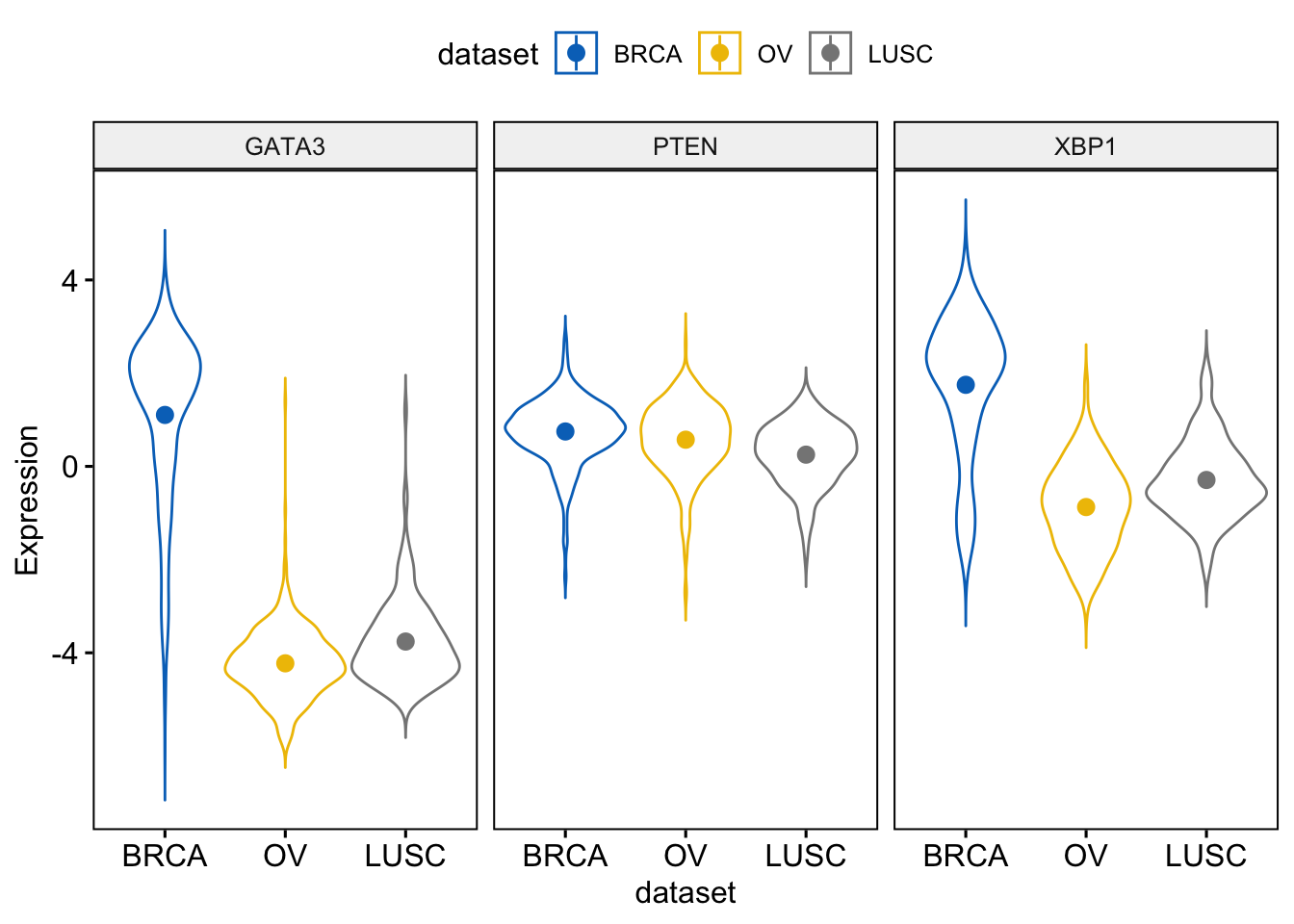
We add quantiles
> ggviolin(expr, x = "dataset",
+            y = c("GATA3", "PTEN", "XBP1"),
+            combine = TRUE, draw_quantiles = c(.025,.5,.75,.975),
+            color = "dataset", palette = "jco",
+            ylab = "Expression",
+            add = "boxplot")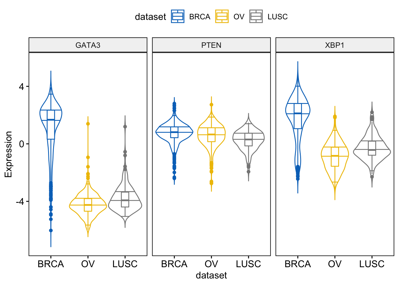
Density plots
To visualize the distribution as a density plot,
> ggdensity(expr,
+        x = c("GATA3", "PTEN",  "XBP1"),
+        y = "..density..",
+        combine = TRUE,                  # Combine the 3 plots
+        xlab = "Expression",
+        add = "median",                  # Add median line.
+        rug = TRUE                       # Add marginal rug
+ )
Change color and fill by dataset
> ggdensity(expr,
+        x = c("GATA3", "PTEN",  "XBP1"),
+        y = "..density..",
+        combine = TRUE,                  # Combine the 3 plots
+        xlab = "Expression",
+        add = "median",                  # Add median line.
+        rug = TRUE,                      # Add marginal rug
+        color = "dataset",
+        fill = "dataset",
+        palette = "jco"
+ )
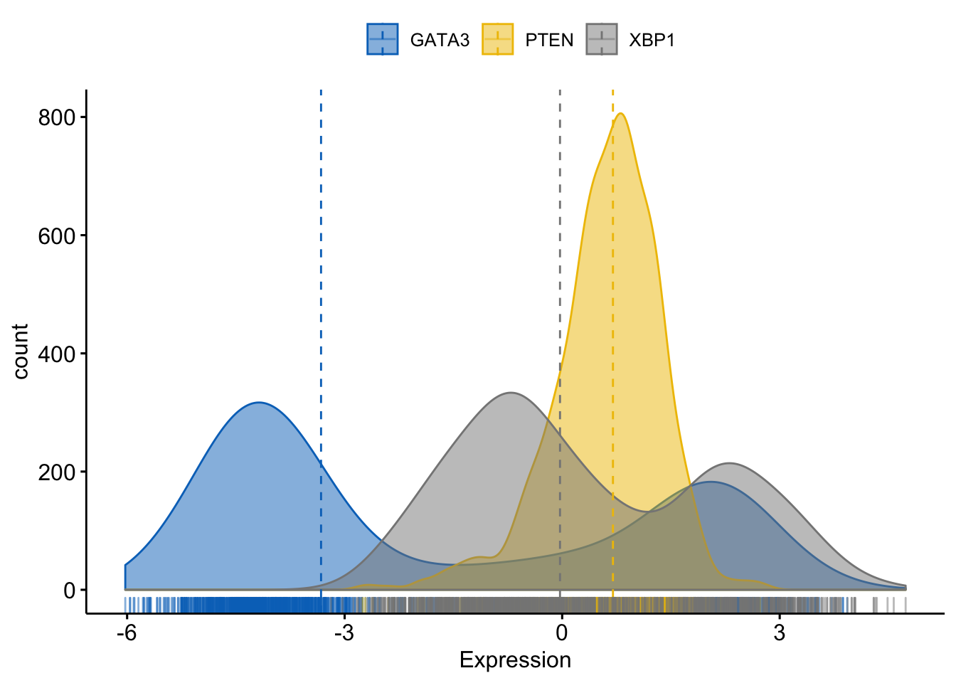
Merging all the plots in one figure
> ggdensity(expr,
+        x = c("GATA3", "PTEN",  "XBP1"),
+        y = "..count..",
+        color = ".x.", fill = ".x.",     # color and fill by x variables
+        merge = TRUE,                    # Merge the 3 plots
+        xlab = "Expression",
+        add = "median",                  # Add median line.
+        rug = TRUE ,                     # Add marginal rug
+        palette = "jco"                  # Change color palette
+ )
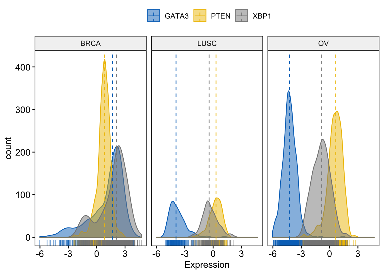
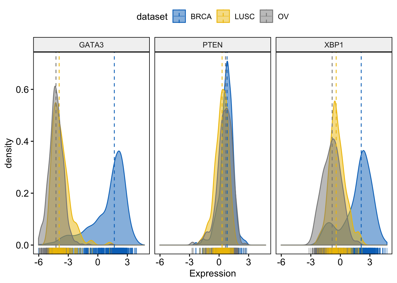
Facet by dataset
> ggdensity(expr,
+        x = c("GATA3", "PTEN",  "XBP1"),
+        y = "..count..",
+        color = ".x.", fill = ".x.",
+        facet.by = "dataset",            # Split by "dataset" into multi-panel
+        merge = TRUE,                    # Merge the 3 plots
+        xlab = "Expression",
+        add = "median",                  # Add median line.
+        rug = TRUE ,                     # Add marginal rug
+        palette = "jco"                  # Change color palette
+ )