How can I select the best SARIMA model

The aim of this note is to show, using a real data, how to select the best a SARIMA model for a given time series.
I won’t remind here the theory behind SARIMA models. You can either come to my class to learn more about time series 😎😎😎 or read the following books
- Robert H. Shumway and David S. Stoffer, Time Series Analysis and Its Applications With R Examples, Springer, 2016
- Avishek Pal and PKS Prakash, Practical Time Series Analysis, Birmingham - Mumbai, 2017.
I will use in this tutorial
- the data departures available in fpp2 package and I will the series permanent. It’s about Overseas departures from Australia and I will be using the monthly number permanent departures from January 1976 - November 2016.
- R packages such as fpp2, forecast, urca and ggplot2
I start then by importing the data from fpp2 package and representing it in a graph

> library(fpp2)
> library(ggplot2)
> data("departures")
> x=departures[,1]
> x%>%autoplot()+theme_bw()+xlab("Years")+ ylab("Departures")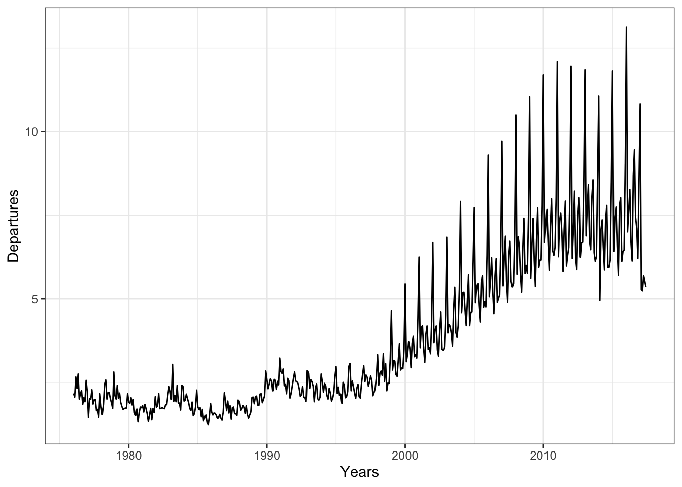

We can quickly notice that there’s a trend-cycle behavior and some kind of seasonality. I will firstly use auto.arima, from forecast package, command to check quickly if this kind of data can be fitted using SARIMA models. I the estimated AIC is non-negative and if the log likelihood is negative we can conclude that SARIMA models can be good for this data. I will also use auto.sarima command to get an idea about the values of $d$, $D$ and $T$.

> library(forecast)
> m0<-auto.arima(x)
> m0

## Series: x 
## ARIMA(0,1,1)(0,1,1)[12] 
## 
## Coefficients:
##           ma1     sma1
##       -0.5216  -0.4012
## s.e.   0.0436   0.0412
## 
## sigma^2 estimated as 0.1002:  log likelihood=-130.45
## AIC=266.9   AICc=266.95   BIC=279.46

I can first notice that I can continue using SARIMA models that fits with this data. I won’t use the previous estimated model by auto.arima because I’m not sure that I’m selecting the best model using the auto.arima command. I will differentiate the series until I obtain stationary. Once this step is done, I will run a selection procedure that we provide the best model adjusting my data that I can use it to make predictions.
I will first represent the process $(1-B)(1-B^12)X_t$ obtained by differentiating my original time series $X_t$.

> library(latex2exp)
> x%>%diff(12)%>%diff(1)%>%autoplot()+theme_bw()+ylab(TeX("$(1-B)(1-B^2)X_t$}$"))+xlab("")

I can notice from the previous graph that $(1-B)(1-B^12)X_t$ has a stationary behavior. I will confirm this using ADF test and KPSS test too. Both tests can be performed using respectively the commands ur.df and ur.kpss.
Since we notice in the previous graph that the time series $(1-B)(1-B^12)X_t$ has no trend and no drift. I will then choose the type="none" for the ADF test and the type=mu for the KPSS test.

> library(urca)
> t1=x%>%diff(12)%>%diff(1)%>%ur.df(lags = 6,type="none")
> summary(t1)

## 
## ############################################### 
## # Augmented Dickey-Fuller Test Unit Root Test # 
## ############################################### 
## 
## Test regression none 
## 
## 
## Call:
## lm(formula = z.diff ~ z.lag.1 - 1 + z.diff.lag)
## 
## Residuals:
##      Min       1Q   Median       3Q      Max 
## -1.97024 -0.18372  0.00008  0.17017  1.33122 
## 
## Coefficients:
##             Estimate Std. Error t value Pr(>|t|)    
## z.lag.1     -2.38348    0.20765 -11.478  < 2e-16 ***
## z.diff.lag1  0.86632    0.19067   4.544 7.04e-06 ***
## z.diff.lag2  0.64170    0.16989   3.777 0.000179 ***
## z.diff.lag3  0.55904    0.14808   3.775 0.000180 ***
## z.diff.lag4  0.47815    0.12148   3.936 9.54e-05 ***
## z.diff.lag5  0.27783    0.08903   3.121 0.001915 ** 
## z.diff.lag6  0.11445    0.04853   2.359 0.018753 *  
## ---
## Signif. codes:  0 '***' 0.001 '**' 0.01 '*' 0.05 '.' 0.1 ' ' 1
## 
## Residual standard error: 0.3351 on 471 degrees of freedom
## Multiple R-squared:  0.7267, Adjusted R-squared:  0.7226 
## F-statistic: 178.9 on 7 and 471 DF,  p-value: < 2.2e-16
## 
## 
## Value of test-statistic is: -11.4782 
## 
## Critical values for test statistics: 
##       1pct  5pct 10pct
## tau1 -2.58 -1.95 -1.62

First, I notice that the regression in the ADF test is significant ; a small p-value, an $R^2$ close to 1 and the coefficients are significant. The value of test-statistic is -11.4782. It’s very smaller that the critical value corresponding to the p-value 1%. Then the p-value of the hypothesis test: \[H_0\,:\, \phi=0\;\mbox{ vs }\;$H_1\,:\, \phi<0\] Hence $H_0$ is rejected and then I can conclude that $(1-B)(1-B^12)X_t$ can be considered as a stationary process.
Let’s now perform a KPSS test

> library(urca)
> t2=x%>%diff(12)%>%diff(1)%>%ur.kpss(type="mu")
> summary(t2)

## 
## ####################### 
## # KPSS Unit Root Test # 
## ####################### 
## 
## Test is of type: mu with 5 lags. 
## 
## Value of test-statistic is: 0.0221 
## 
## Critical value for a significance level of: 
##                 10pct  5pct 2.5pct  1pct
## critical values 0.347 0.463  0.574 0.739

The value of the test-statistic is .0221 smaller than the critical value corresponding to the p-value 10%. We can also conclude that $(1-B)(1-B^12)X_t$ can be considered as a stationary process.
I can then conclude that $d=D=1$ and $T=12$. Let’s notice that $T=12$ is expected since we’re dealing with monthly data.
In the next step I will determine the possible values of $p$, $P$, $q$ and $Q$. I will ACF to determine the couples $(q,Q)$ and I will use PACF to determine the couples $(p,P)$.

> x%>%diff(12)%>%diff(1)%>%ggAcf()+theme_bw()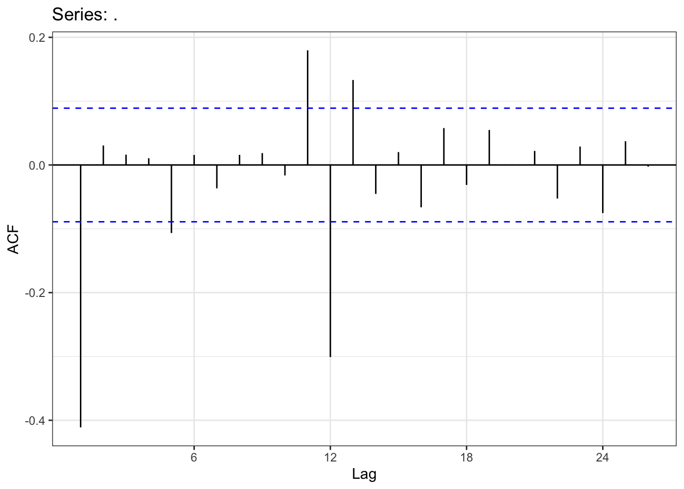

I can deduce from the previous graph that the ACF are equal to zero from the order 14 and these ACF are decreasing to zero. Then $q+12Q\leq 13$. Let’s recall that $q+12Q$ is the degree of the MA operator.
Let’s now draw the PACF

> x%>%diff(12)%>%diff(1)%>%ggPacf()+theme_bw()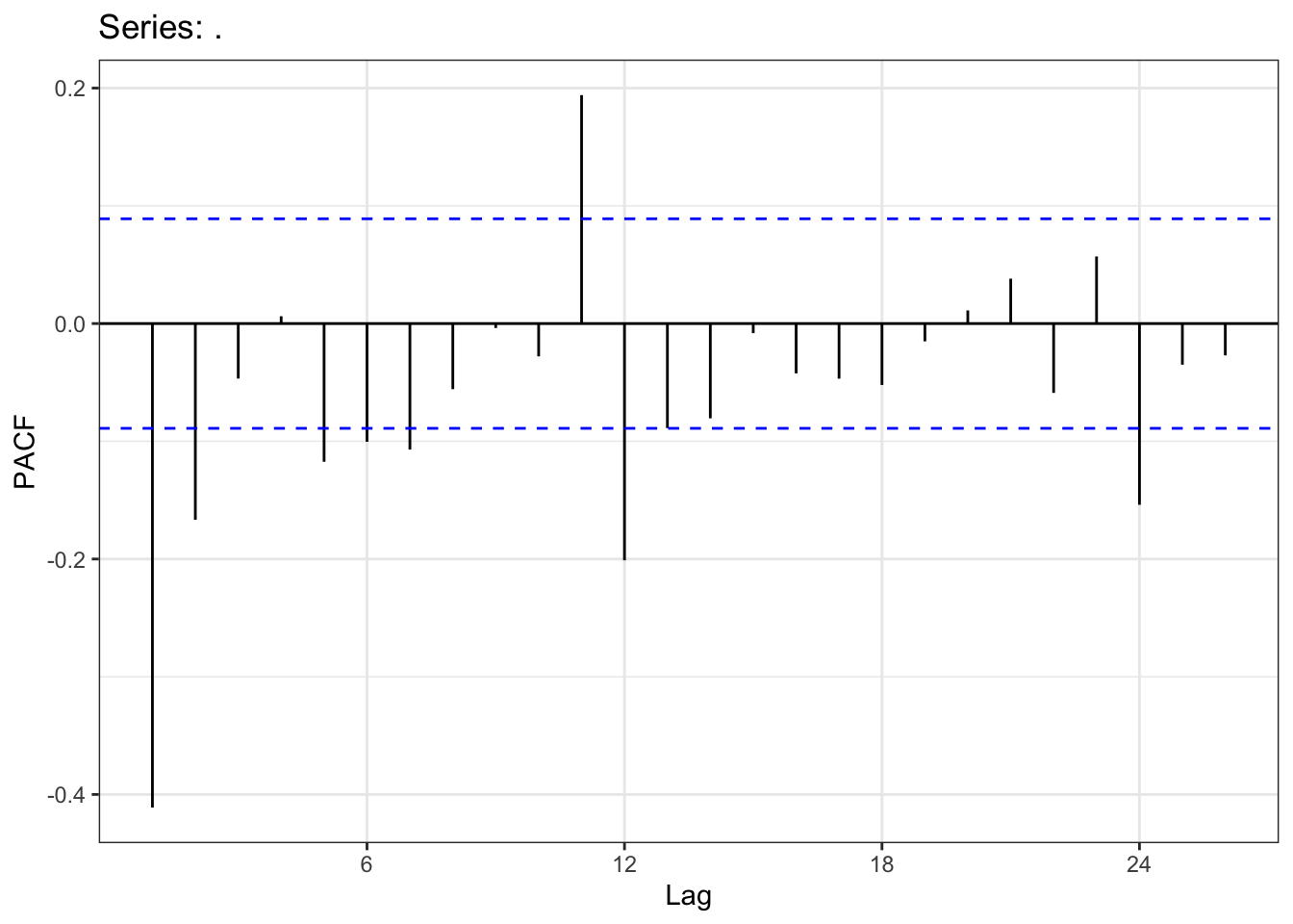

I will then have the same conclusion as in the ACF and I will choose the couples $p+12P$ such that $p+12P\leq 13$.
I will now start the selection procedure. I will first construct a matrix with the possibles values of $p$, $d$, $q$, $P$, $D$, $Q$ and $T$. Each row corresponds to each case. In the total we have to estimate 256. It’s a lot but it just takes about 10 to 15 minutes to get all results. I will then eliminate the models with negative AIC and then I will eliminate the models that generate not white noise residuals.
Construction of the matrix of the parameters $p$, $d$, $q$, $P$, $D$, $Q$ and $T$:

> qQ=list()
> for(i in 1:14) qQ[[i]]=c(i-1,0)
> qQ[[15]]=c(0,1)
> qQ[[16]]=c(1,1)
> pP=qQ
> 
> dt_params=c()
> for(i in 1:16){
+   for(j in 1:16){
+     temp=c(pP[[i]][1],1,qQ[[j]][1],pP[[i]][2],1,
+            qQ[[j]][2],12)
+     dt_params=rbind(temp,dt_params)
+   }
+ }
> colnames(dt_params)=c("p","d","q","P","D","Q","T")
> rownames(dt_params)=1:256

Estimating the models now. You can notice that I have added the command try in the loop. Indeed I didn’t want that the loops stops when the estimation algorithm doesn’t converge. It will just provide a void object.

> models=vector("list",256)
> for(i in 1:256){
+   try(models[[i]]<-Arima(x,order = dt_params[i,1:3],
+                     seasonal = list(order=dt_params[i,4:6],period=12),
+                     lambda = NULL))
+ }

I will now check the residuals, I had constructed a test that I use to eliminate the models that not-white-noise residual. Indeed, I perform a Portemanteau test with lags from 1 to 10. The model is rejected if at least one p-value from the later test is smaller than the significance level 5%. I will be using the command Box.test.2 from caschrono package.

> library(caschrono)
> aa=rep(NA,256)
> for(i in 1:256){
+   if(length(models[[i]]$residuals)>1){
+     a=Box.test.2(x = models[[i]]$residuals,nlag = 10,type = "Box-Pierce")
+     z=prod(1-(a[,2]<.05))
+     if(z==1) aa[i]="y"
+     else aa[i]="n"
+   }
+  
+ }
> dt_params2=data.frame(dt_params)
> dt_params2$residuals=aa

Hence the object aa will tell us if the white-noise test was successful or not.
I will now create a vector aic that contains the AIC of the estimated models

> aic=rep(NA,256)
> model_names=rep(NA,256)
> for(i in 1:256){
+   if(length(models[[i]]$aic)>0){
+     aic[i]=models[[i]]$aic
+     model_names[i]=as.character(models[[i]])
+   }
+ }
> dt_params2$aic=aic
> dt_params2$model=model_names

Here’s a table with the all previous results

> library(DT)
> dt_params2$aic=round(dt_params2$aic,4)
> dt_params2=na.omit(dt_params2)
> datatable(dt_params2,rownames = F)

Let’s notice that we obtain here models with AIC smaller than the model selected by auto.arima. We will then select the models with AIC smaller than 260 and we display them all.

> i=as.numeric(rownames(dt_params2)[which(dt_params2$aic<260)])
> res=sapply(i, function(x)as.character(models[[x]]))
> res

##  [1] "ARIMA(13,1,11)(0,1,0)[12]" "ARIMA(12,1,1)(0,1,1)[12]" 
##  [3] "ARIMA(12,1,11)(0,1,0)[12]" "ARIMA(10,1,13)(0,1,0)[12]"
##  [5] "ARIMA(8,1,13)(0,1,0)[12]"  "ARIMA(8,1,12)(0,1,0)[12]" 
##  [7] "ARIMA(7,1,13)(0,1,0)[12]"  "ARIMA(7,1,12)(0,1,0)[12]" 
##  [9] "ARIMA(6,1,1)(0,1,1)[12]"   "ARIMA(6,1,13)(0,1,0)[12]" 
## [11] "ARIMA(5,1,1)(0,1,1)[12]"   "ARIMA(5,1,13)(0,1,0)[12]" 
## [13] "ARIMA(4,1,1)(0,1,1)[12]"   "ARIMA(4,1,13)(0,1,0)[12]" 
## [15] "ARIMA(3,1,1)(0,1,1)[12]"   "ARIMA(2,1,1)(0,1,1)[12]"

I will now reject the models that contain non significant coefficient. To do so, I will use t_stat from cashchrono package that performs a $t-$test for each coefficient.

> x_test=sapply(i, function(x)t_stat(models[[x]]))
> bb=rep(NA,16)
> for(j in 1:16){
+   temp=t(x_test[[j]])[,2]
+   z=prod((temp<.05))
+   bb[j]=z
+ }
> bb

##  [1] 0 0 0 0 0 0 0 0 0 0 0 0 0 0 1 1

Only the last two models have then all their coefficients significant. These models are

> models[[i[length(i)-1]]]

## Series: x 
## ARIMA(3,1,1)(0,1,1)[12] 
## 
## Coefficients:
##          ar1     ar2     ar3      ma1     sma1
##       0.4400  0.2009  0.1103  -0.9706  -0.3790
## s.e.  0.0481  0.0504  0.0489   0.0162   0.0431
## 
## sigma^2 estimated as 0.0973:  log likelihood=-122.33
## AIC=256.66   AICc=256.84   BIC=281.77

> models[[i[length(i)]]]

## Series: x 
## ARIMA(2,1,1)(0,1,1)[12] 
## 
## Coefficients:
##          ar1     ar2      ma1     sma1
##       0.4580  0.2415  -0.9636  -0.3678
## s.e.  0.0484  0.0478   0.0184   0.0433
## 
## sigma^2 estimated as 0.09814:  log likelihood=-124.87
## AIC=259.74   AICc=259.87   BIC=280.66

The best model is then

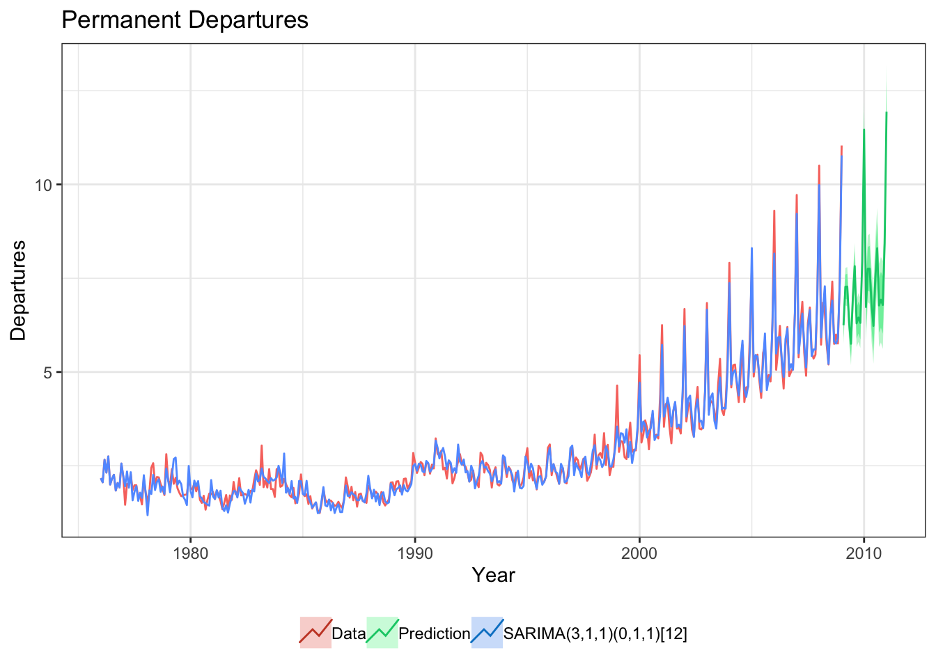
> as.character(models[[i[length(i)-1]]])

## [1] "ARIMA(3,1,1)(0,1,1)[12]"

Let’s now represent the data, the fitted values by the selected model and a forecast provided by it.

> x_tr <- window(x,end=2009) 
> fit <- Arima(x_tr,order = c(3,1,1),
+                     seasonal = list(order=c(0,1,1),period=12),
+                     lambda = NULL)
> f_fit<-forecast(fit)
> 
> autoplot(x_tr, series="Data") + 
+   autolayer(fit$fitted, series="SARIMA(3,1,1)(0,1,1)[12]") +
+   autolayer(f_fit, series="Prediction") +
+   xlab("Year") + ylab("Departures") + ggtitle("Permanent Departures") + theme_bw()+theme(legend.title = element_blank(),legend.position = "bottom")