Spark with RStudio
Spark
![]()
Apache Spark is a powerful open source processing engine built around speed, ease of use, and sophisticated analytics. It was originally developed at UC Berkeley in 2009.
Spark can be 100x faster than Hadoop for large scale data processing by exploiting in memory computing and other optimization.
We can now use easily Spark from RStudio. Its latest includes integrated support for Spark and the sparklyr package, including tools for:
- Creating and managing Spark connections
- Browsing the tables and columns of Spark DataFrames
- Previewing the first 1,000 rows of Spark DataFrames
To learn more about it visit https://spark.rstudio.com and here also some other video tutorial very interesting to watch: https://www.rstudio.com/resources/webinars/
This is how we can connect Spark to RStudio
Connecting Spark to RStudio
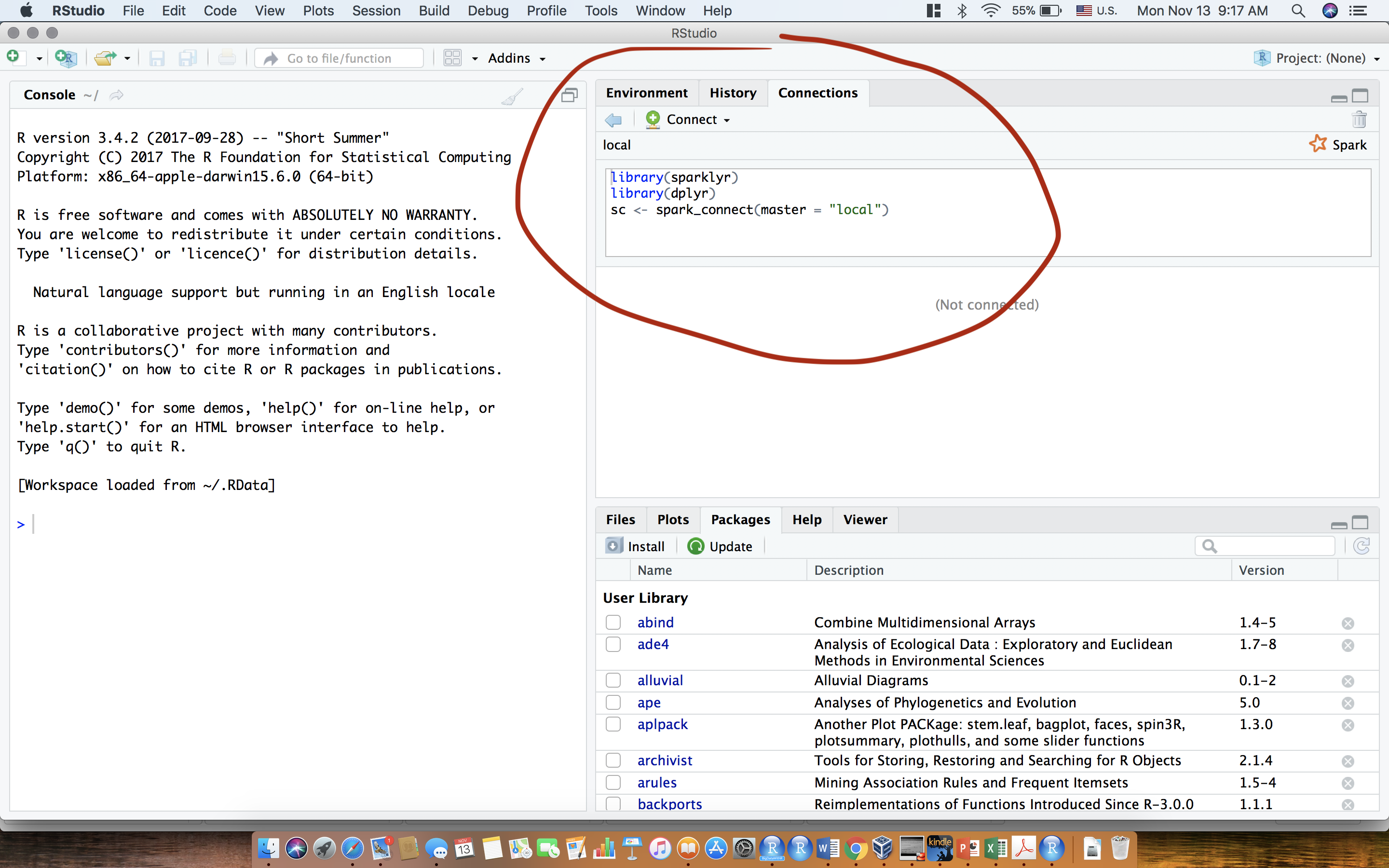


Creating your first Spark session
We will use a custom configuration for the sparklyr connection, we are requesting:
- 16 gigabytes of memory for the
driver - Make 80% of the memory accessible to use during the analysis
Let’s now import the airline_20MM.csv file. Let’s recall that it’s a data with 20,000,000 rows and the size of the file is ~ 1.5GB
> ptm=proc.time()
> airline_20MM_sp <- spark_read_csv(sc, "airline_20MM","airline_20MM.csv")
> proc.time()-ptm
   user  system elapsed
  0.279   0.289 132.128
You can check some information about your data like you usually do in R
> colnames(airline_20MM_sp)
 [1] "Year"              "Month"             "DayofMonth"        "DayOfWeek"
 [5] "DepTime"           "CRSDepTime"        "ArrTime"           "CRSArrTime"
 [9] "FlightNum"         "ActualElapsedTime" "CRSElapsedTime"    "AirTime"
[13] "ArrDelay"          "DepDelay"          "Distance"          "TaxiIn"
[17] "TaxiOut"           "Cancelled"         "Diverted"          "CarrierDelay"
[21] "WeatherDelay"      "NASDelay"          "SecurityDelay"     "LateAircraftDelay"
[25] "IsArrDelayed"      "IsDepDelayed"
We will show now how to import the Airline 20M data into R using Spark and RStudio.
We will compute the number of flights by year and draw the bar-chart
> ptm=proc.time()
> nbre_flights_year <- airline_20MM_sp %>%
+   group_by(Year) %>%
+   summarise(count = n())
> proc.time()-ptm
   user  system elapsed
  0.007   0.002   0.007
> ptm=proc.time()
> ggplot(nbre_flights_year, aes(x=Year,y=count))+
+   geom_bar(stat = "identity")+xlab("Year")+ylab("Number of flights")+theme_bw()
> proc.time()-ptm
   user  system elapsed
0.260 0.041 2.135 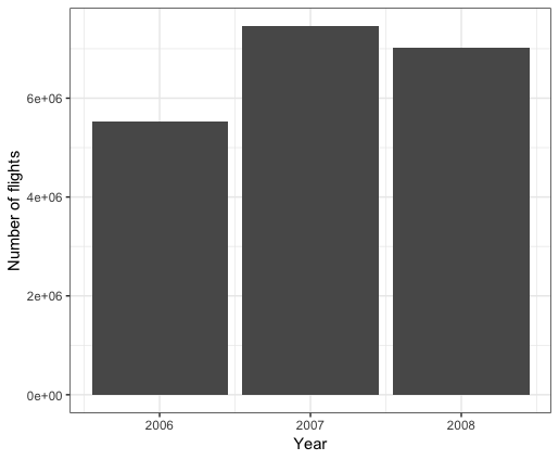
Setting up the lastest version of Spark with RStudio (Local mode)
We will show here how we can work with Spark and RStudio in a local mode. It’s an excellent way to learn and test how Spark works and it gives a nice environment to analyse statistically large datasets.
We will first load the packages and configure the Spark connection in the local mode
> library(sparklyr)
> library(dplyr)
We need then to configure the Spark connection
> conf <- spark_config()
> conf
$spark.env.SPARK_LOCAL_IP.local
[1] "127.0.0.1"

$sparklyr.connect.csv.embedded
[1] "^1.*"

$spark.sql.catalogImplementation
[1] "hive"

$sparklyr.connect.cores.local
[1] 4

$spark.sql.shuffle.partitions.local
[1] 4

attr(,"config")
[1] "default"
attr(,"file")
[1] "/Library/Frameworks/R.framework/Versions/3.5/Resources/library/sparklyr/conf/config-template.yml"
We will tell to R that we will be using the available cores. They are by default 4.
> conf$`sparklyr.cores.local` <- 4We will be also using the limit RAM available memory in the computer minus what would be needed for OS operations.
> conf$`sparklyr.shell.driver-memory` <- "16G"And we will tell to R that we need 90% of the fraction of the memory.
> conf$spark.memory.fraction <- 0.9Before connecting Spark, let’s check latest available version of Spark

Let’s then install the 2.3.2 Spark version from RStudio. Of course, before this installation you need also to update your Java version: https://www.java.com
> spark_install(version = "2.3.2")
Installing Spark 2.3.2 for Hadoop 2.7 or later.
Downloading from:
- 'https://archive.apache.org/dist/spark/spark-2.3.2/spark-2.3.2-bin-hadoop2.7.tgz'
Installing to:
- '~/spark/spark-2.3.2-bin-hadoop2.7'
trying URL 'https://archive.apache.org/dist/spark/spark-2.3.2/spark-2.3.2-bin-hadoop2.7.tgz'
Content type 'application/x-gzip' length 225875602 bytes (215.4 MB)
==================================================
downloaded 215.4 MB

Installation complete.
We can now connect Spark to R
> sc <- spark_connect(master = "local",
+                     version = "2.3.2",
+                     config = conf)
By clicking on SparkUI as shown below the Spark workflow will be opened in your favorite web browser
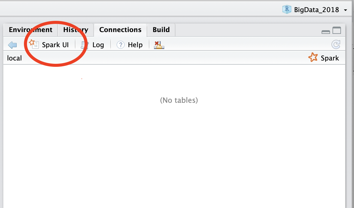
Here’s then the Spark workflow
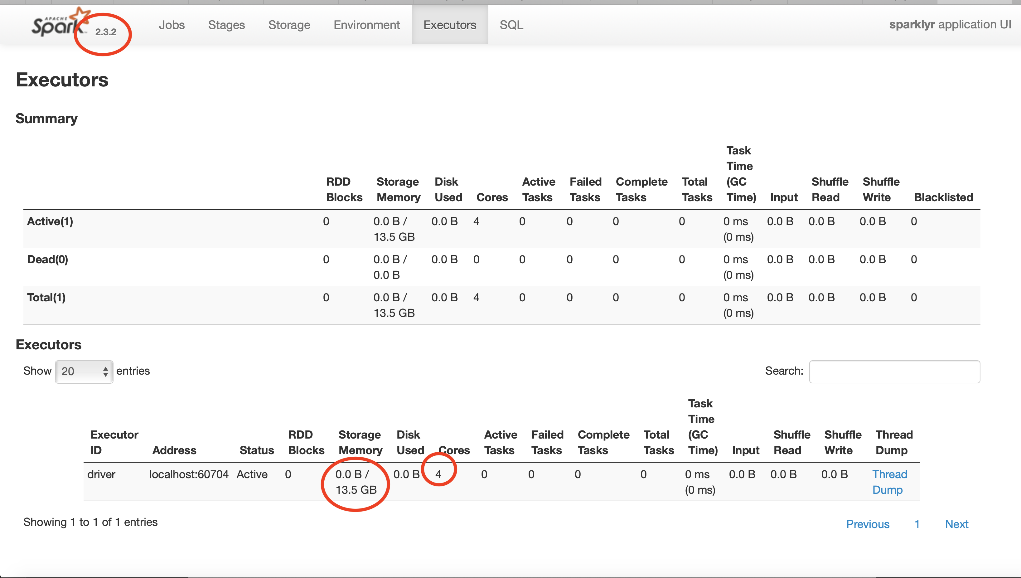
There are many other modes to run Spark from RStudio: YARN, Cluster Mode, Standalone mode. You learn more about it visit: https://spark.rstudio.com/guides/connections/
Spark Machine Learning Library (MLlib)
We will show in this section how can we use some classical Machine Learning algorithm work with Spark connected to RStudio.
Data preparation
We will be using in this example census_income.csv available in https://www.kaggle.com/dhafer/census-income-data-big-data-class
Let’s import the data
> ptm=proc.time()
> census_tbl <- spark_read_csv(sc, "census_inc","census_income.csv",overwrite = T)
> proc.time()-ptm
   user  system elapsed
  0.222   0.022   4.492
Let’s see a preview of the data
> census_tbl%>%head
# Source: spark<?> [?? x 15]
    age workclass fnlwgt education educationnum maritalstatus occupation relationship race
* <int> <chr>      <int> <chr>            <int> <chr>         <chr>      <chr>        <chr>
1    39 " State-…  77516 " Bachel…           13 " Never-marr… " Adm-cle… " Not-in-fa… " Wh…
2    50 " Self-e…  83311 " Bachel…           13 " Married-ci… " Exec-ma… " Husband"   " Wh…
3    38 " Privat… 215646 " HS-gra…            9 " Divorced"   " Handler… " Not-in-fa… " Wh…
4    53 " Privat… 234721 " 11th"              7 " Married-ci… " Handler… " Husband"   " Bl…
5    28 " Privat… 338409 " Bachel…           13 " Married-ci… " Prof-sp… " Wife"      " Bl…
6    37 " Privat… 284582 " Master…           14 " Married-ci… " Exec-ma… " Wife"      " Wh…
# ... with 6 more variables: sex <chr>, capitalgain <int>, capitalloss <int>,
#   hoursperweek <int>, nativecountry <chr>, label <chr>
We can for example arrange it according to the age and select some variables to be used later for our next analysis.
> census_tbl%>%select(age,capitalgain,capitalloss,hoursperweek,sex,nativecountry)%>% arrange(age) %>% head
# Source:     spark<?> [?? x 6]
# Ordered by: age
    age capitalgain capitalloss hoursperweek sex       nativecountry
* <int>       <int>       <int>        <int> <chr>     <chr>
1    17           0           0           12 " Male"   " United-States"
2    17           0           0           40 " Male"   " United-States"
3    17        1055           0           24 " Male"   " United-States"
4    17           0           0           12 " Female" " United-States"
5    17           0           0           48 " Male"   " Mexico"
6    17           0           0           10 " Male"   " United-States"
We will now create a code to create a new dataset with the variables: Sex, hoursperweek and two new variables: + nativecountry yes/no + Capital: it’s positive if there’s a gain in the capital and negative otherwise.
We then select the variables and create a new capitalloss variable equal to minus the previous capitalloss variable
> census_tbl1<-census_tbl%>%select(age,capitalgain,capitalloss,hoursperweek,nativecountry,sex)%>%mutate(capitalloss2=-capitalloss)I remove then capitalloss variable
> census_tbl1<-census_tbl1%>%select(-capitalloss)Let’s now reshape the data to get only one capitalgain variable
> library(tidyr)
> census_dt=as.data.frame(census_tbl1)
> census_dt<-gather(census_dt, variable, value, -c(age,hoursperweek,nativecountry,sex))
> census_dt%>%head
  age hoursperweek  nativecountry     sex    variable value
1  39           40  United-States    Male capitalgain  2174
2  50           13  United-States    Male capitalgain     0
3  38           40  United-States    Male capitalgain     0
4  53           40  United-States    Male capitalgain     0
5  28           40           Cuba  Female capitalgain     0
6  37           40  United-States  Female capitalgain     0
We nee now to recode the nativecountry variable: Either in USA (yes) or (no) if others.
> census_dt=census_dt%>%mutate(nativecountry2 = (nativecountry==" United-States"))
> census_dt=census_dt%>%select(-nativecountry)
> census_dt=census_dt%>%mutate(nativecountry2=as.factor(nativecountry2))
> census_dt%>%mutate(nativecountry=fct_recode(nativecountry2,"yes"="TRUE","no"="FALSE"))%>%head
  age hoursperweek     sex    variable value nativecountry2 nativecountry
1  39           40    Male capitalgain  2174           TRUE           yes
2  50           13    Male capitalgain     0           TRUE           yes
3  38           40    Male capitalgain     0           TRUE           yes
4  53           40    Male capitalgain     0           TRUE           yes
5  28           40  Female capitalgain     0          FALSE            no
6  37           40  Female capitalgain     0           TRUE           yes
> census_dt<-census_dt%>%mutate(nativecountry=fct_recode(nativecountry2,"yes"="TRUE","no"="FALSE"))
> census_dt=census_dt%>%select(-nativecountry2)
> census_dt%>%head
  age hoursperweek     sex    variable value nativecountry
1  39           40    Male capitalgain  2174           yes
2  50           13    Male capitalgain     0           yes
3  38           40    Male capitalgain     0           yes
4  53           40    Male capitalgain     0           yes
5  28           40  Female capitalgain     0            no
6  37           40  Female capitalgain     0           yes
and we will copy it into Spark environment
> census_tbl<-copy_to(sc,census_dt,"census_dt",overwrite = T)
# Source: spark<census_dt> [?? x 6]
     age hoursperweek sex       variable    value nativecountry
 * <int>        <int> <chr>     <chr>       <int> <chr>
 1    39           40 " Male"   capitalgain  2174 yes
 2    50           13 " Male"   capitalgain     0 yes
 3    38           40 " Male"   capitalgain     0 yes
 4    53           40 " Male"   capitalgain     0 yes
 5    28           40 " Female" capitalgain     0 no
 6    37           40 " Female" capitalgain     0 yes
 7    49           16 " Female" capitalgain     0 no
 8    52           45 " Male"   capitalgain     0 yes
 9    31           50 " Female" capitalgain 14084 yes
10    42           40 " Male"   capitalgain  5178 yes
# ... with more rows
Data Visualization
We will plot here the scatter plot between the age and the capitalgain according to the categorical variables sex and native country.
> ptm=proc.time()
> p<-ggplot(census_tbl, aes(age, value)) +
+   geom_point(alpha = 1/2) +
+   scale_size_area(max_size = 2)+
+   facet_grid(sex~nativecountry)
> p+theme_bw()
> proc.time()-ptm
   user  system elapsed
2.057 0.128 2.542 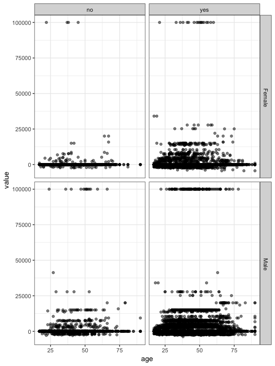
Linear models with MLib
We will make a partition of the data into a train and test data
> census_pt1 <- census_tbl %>%
+   sdf_partition(training = 0.7, test = 0.3, seed = 1099)
We estimate then the linear model as follows
> fit <- census_pt1$training %>%
+   ml_linear_regression(response = "value",
+                        features = c("age","sex","hoursperweek","nativecountry"))
Here the estimation of the coefficients
> summary(fit)
Deviance Residuals:
    Min      1Q  Median      3Q     Max
-5649.9  -728.3  -480.2  -214.6 99971.1

Coefficients:
      (Intercept)               age         sex_ Male      hoursperweek nativecountry_yes
      -1082.25907          18.34806         205.00438          16.43393          67.50759

R-Squared: 0.005063
Root Mean Squared Error: 5139
And the p-values of the coefficients
> round(fit$summary$p_values,4)
[1] 0.0000 0.0000 0.0001 0.0000 0.3891
Let’s draw a scatter plot with the predicted values on the test data and the real values and let’s check how can is the estimated model
> census_pred<-ml_predict(fit, census_pt1$test)
> census_pred
# Source: spark<?> [?? x 7]
     age hoursperweek sex       variable     value nativecountry prediction
 * <int>        <int> <chr>     <chr>        <int> <chr>              <dbl>
 1    17            5 " Female" capitalloss2     0 yes                -621.
 2    17            5 " Female" capitalloss2     0 yes                -621.
 3    17            5 " Male"   capitalloss2     0 yes                -416.
 4    17            5 " Male"   capitalloss2     0 yes                -416.
 5    17            6 " Female" capitalloss2     0 yes                -604.
 6    17            7 " Female" capitalgain      0 yes                -588.
 7    17            8 " Female" capitalgain      0 yes                -571.
 8    17            8 " Female" capitalgain      0 yes                -571.
 9    17            8 " Female" capitalloss2     0 yes                -571.
10    17            8 " Female" capitalloss2     0 yes                -571.
# ... with more rows
And we draw the plot Real values x Predicted.
> p<-ggplot(census_pred, aes(value, prediction)) +
+   geom_point(alpha = 1/2) +
+   scale_size_area(max_size = 2)+
+   facet_grid(sex~nativecountry)
> p+theme_bw()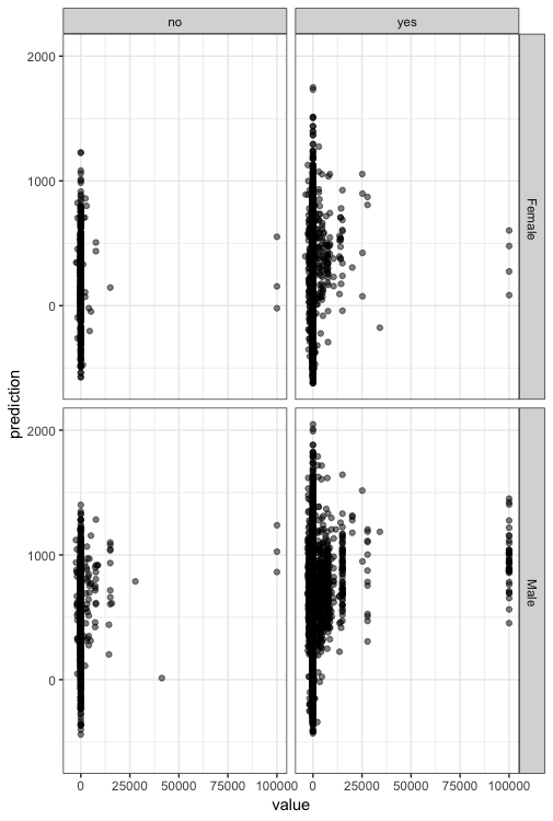
Logistic models
Let us consider in this example the famous titanic data. This data is available in this link : https://github.com/rstudio/sparkDemos. The data that I will be using is under: dev/titanic/. You need then to put the folder titanic-parquet in your working folder in R.
We will now load the needed libraries, set up a local Spark connection and import the data
> library(sparklyr)
> library(dplyr)
> library(tidyr)
> library(titanic)
> library(ggplot2)
> library(purrr)
> sc <- spark_connect(master = "local", version = "2.3.2")
> spark_read_parquet(sc, name = "titanic", path = "titanic-parquet")
# Source: spark<titanic> [?? x 12]
   PassengerId Survived Pclass Name  Sex     Age SibSp Parch Ticket  Fare Cabin
 *       <int>    <int>  <int> <chr> <chr> <dbl> <int> <int> <chr>  <dbl> <chr>
 1           1        0      3 Brau… male     22     1     0 A/5 2…  7.25 NA
 2           2        1      1 Cumi… fema…    38     1     0 PC 17… 71.3  C85
 3           3        1      3 Heik… fema…    26     0     0 STON/…  7.92 NA
 4           4        1      1 Futr… fema…    35     1     0 113803 53.1  C123
 5           5        0      3 Alle… male     35     0     0 373450  8.05 NA
 6           6        0      3 Mora… male    NaN     0     0 330877  8.46 NA
 7           7        0      1 McCa… male     54     0     0 17463  51.9  E46
 8           8        0      3 Pals… male      2     3     1 349909 21.1  NA
 9           9        1      3 John… fema…    27     0     2 347742 11.1  NA
10          10        1      2 Nass… fema…    14     1     0 237736 30.1  NA
# ... with more rows, and 1 more variable: Embarked <chr>
> titanic_tbl <- tbl(sc, "titanic")
Let’s show some proprieties of the imported data
- Number of observations
>  titanic_tbl%>%summarise(n())
# Source: spark<?> [?? x 1]
  `n()`
* <dbl>
1 891- Names of the variables
> colnames( titanic_tbl)
 [1] "PassengerId" "Survived"    "Pclass"      "Name"        "Sex"
 [6] "Age"         "SibSp"       "Parch"       "Ticket"      "Fare"
[11] "Cabin"       "Embarked"
Here’s the descriptions of the variables
PassengerIdPassenger IDSurvivedSurvived or no (1=Survived, 0=No)PclassPassenger ClassNameNameSexSexAgeAgeSibSpNumber of Siblings/Spouses AboardParchNumber of Parents/Children AboardTicketTicket NumberFarePassenger FareCabinCabinEmbarkedPort of Embarkation
The target variable
>  titanic_tbl%>%group_by(Survived)%>%summarise(n())
# Source: spark<?> [?? x 2]
  Survived `n()`
*    <int> <dbl>
1        0   549
2        1   342
We would like in this example to predicted the the Survived variable using the variables Pclass, Sex, Age, SibSp, Parch, Fare Embarked and Family_Sizes. The later variable will be computed as the sum of the variable SibSp and Parch.
Let’s then prepare the data before performing the logistic regression. We will then
- Add the variable
Family_Size - Transform
Pclassas a categorical variable - Impute the missing values of the
Agevariable EmbarkRemove a small number of missing records- Save
titanic2_tblinto Spark environment
titanic2_tbl <- titanic_tbl %>%
  mutate(Family_Size = SibSp + Parch + 1L) %>%
  mutate(Pclass = as.character(Pclass)) %>%
  filter(!is.na(Embarked)) %>%
  mutate(Age = if_else(is.na(Age), mean(Age,na.rm=T), Age)) %>%
  sdf_register("titanic2")
Final transformation: create a new variable Family_Sizes as a discretization of the Family_Size variable
titanic_final_tbl <- titanic2_tbl %>%
  mutate(Family_Size = as.numeric(Family_size)) %>%
  sdf_mutate(
    Family_Sizes = ft_bucketizer(Family_Size, splits = c(1,2,5,12))
  ) %>%
  mutate(Family_Sizes = as.character(as.integer(Family_Sizes))) %>%
  sdf_register("titanic_final")
> titanic_final_tbl%>%group_by(Family_Sizes)%>%summarise(n())
# Source: spark<?> [?? x 2]
  Family_Sizes `n()`
* <chr>        <dbl>
1 1              292
2 2               62
3 0              535
We partition the data into a training and a test samples:
> partition <- titanic_final_tbl %>%
+   mutate(Survived = as.numeric(Survived)) %>%
+   select(Survived, Pclass, Sex, Age,  Fare, Embarked, Family_Sizes) %>%
+   sdf_partition(train = 0.75, test = 0.25, seed = 8585)
> train_tbl <- partition$train
> test_tbl <- partition$test
We estimate then the Logistic model:
- We write the formula of the model
- We use the function
ml_logistic_modelto estimate the mode
> ml_formula <- formula(Survived ~ Pclass + Sex + Age + SibSp + Parch + Fare + Embarked + Family_Sizes)
> ptm=proc.time()
> ml_log <- ml_logistic_regression(train_tbl, ml_formula)
> proc.time()-ptm
   user  system elapsed
  0.742   0.021   5.068
We can determine from the ml_log the estimation of the coefficients:
> ml_log$coefficients
   (Intercept)       Pclass_3       Pclass_1       Sex_male            Age
  1.3058880464  -1.0764234487   1.0012170048  -2.6740732527  -0.0412190132
         SibSp          Parch           Fare     Embarked_S     Embarked_C
 -0.0559892796   0.1628601305   0.0002931061  -0.4650343933  -0.3638728288
Family_Sizes_0 Family_Sizes_1
  1.8269143916   1.9686352964
We need also to compute the performance of the prediction of the model. We need then to recall the following definitions: Since we are predicting a binary variable, let’s denote by \(\widehat{y}(t)\) the predicted value of \(y\) using the a prediction model with a given threshold \(t\in [0,1]\). we can then display the following table:
| Gain, \(y=1\) | No Gain, \(y=0\) | |
|---|---|---|
| Positive \(\widehat{y}(t)=1\) | TP\((t)\) \((y=1,\widehat{y}(t)=1)\) | FP\((t)\) \((y=0,\widehat{y}(t)=1)\) |
| Negative \(\widehat{y}(t)=0\) | FN\((t)\) \((y=1,\widehat{y}(t)=0)\) | TN\((t)\) \((y=0,\widehat{y}(t)=0)\) |
Then
- True Positif: TP\((t)=|\{y=1,\widehat{y}(t)=1\}|\)
- True Negatif: TN\((t)=|\{y=0,\widehat{y}(t)=0\}|\)
- False Negatif: FN\((t)=|\{y=1,\widehat{y}(t)=0\}|\) (Type 2 error)
- False Positif: FP\((t)=|\{y=0,\widehat{y}(t)=1\}|\) (Type 1 error)
We can then measure also
- Sensitivity TPR=TP/TP+FN
- Specificity TNR=TN/TN+FP
- Accuracy: (TP+TN)/(P+N).
- TPR: true positive rate (sensitivity) TP/(FP+TP).
- FPR: false positive rate FP/N=FP/(FN+TN)
- FNR: false negative rate FN/P=FN/(FP+TP)
- TNR: true negative rate (Specificity) TN/N=TN/(FN+TN)
We usually also display the Receiver operating characteristic (ROC) curves. They are graphical plots that illustrate the performance of a binary classifier. They visualize the relationship between the true positive rate (TPR) against the false positive rate (FPR).
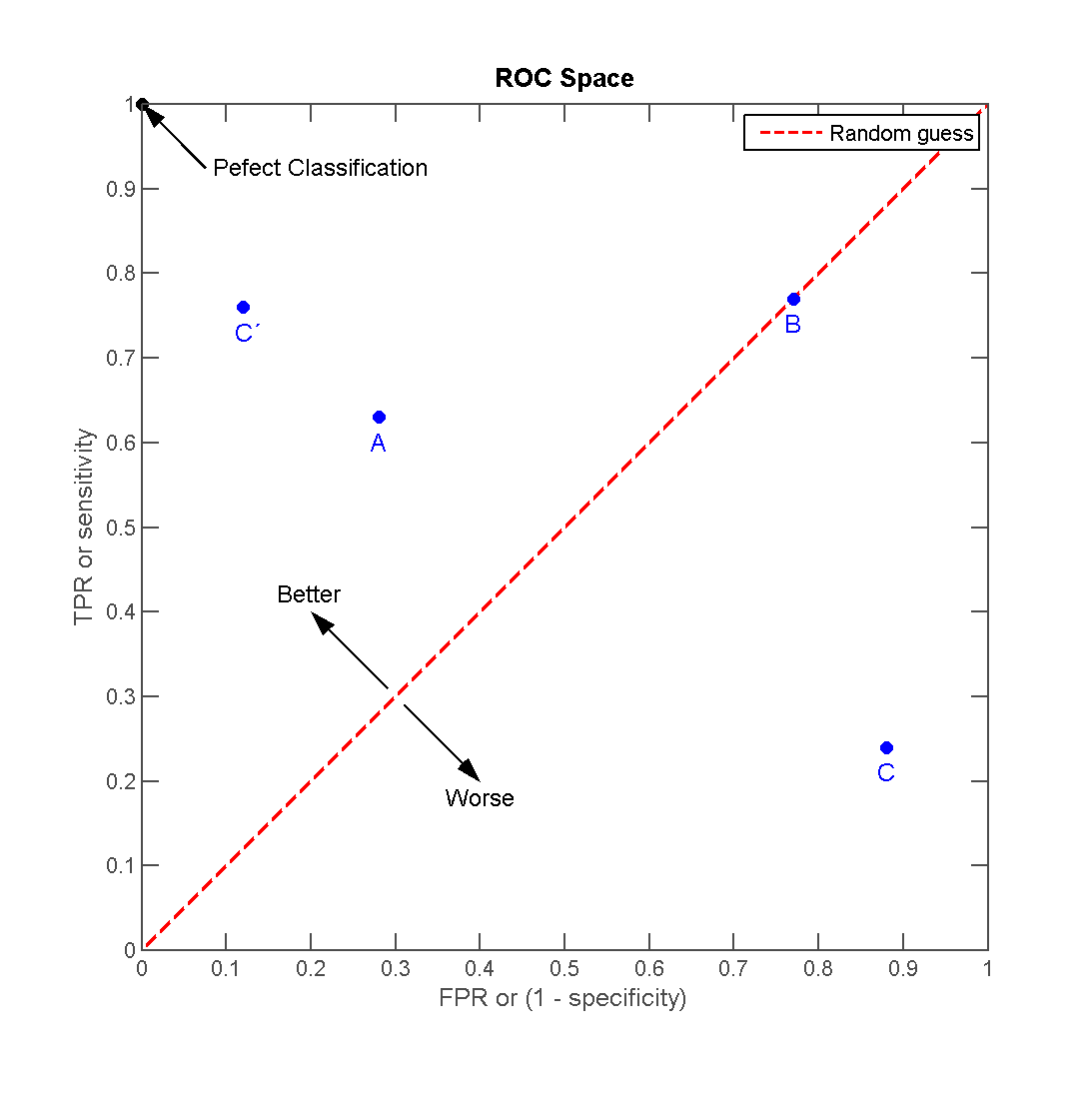
The ideal model perfectly classifies all positive outcomes as true and all negative outcomes as false (i.e. TPR = 1 and FPR = 0).
The area under the curve (AUC) summarizes how good the model is across these threshold points simultaneously. An area of 1 indicates that for any threshold value, the model always makes perfect prediction.
Let’s show then how to draw the ROC curve from the ml_log result.
> d_roc=as.data.frame(ml_log$summary$roc())
> d_roc%>%head
          FPR        TPR
1 0.000000000 0.00000000
2 0.002439024 0.01538462
3 0.002439024 0.03461538
4 0.004878049 0.05000000
5 0.004878049 0.06923077
6 0.004878049 0.08846154
and the ROC curve is
> ggplot(d_roc,aes(x=FPR,y=TPR))+geom_line()+xlab("FPR (1-specificity)")+ylab("TPR (sensitivity)")+theme_bw()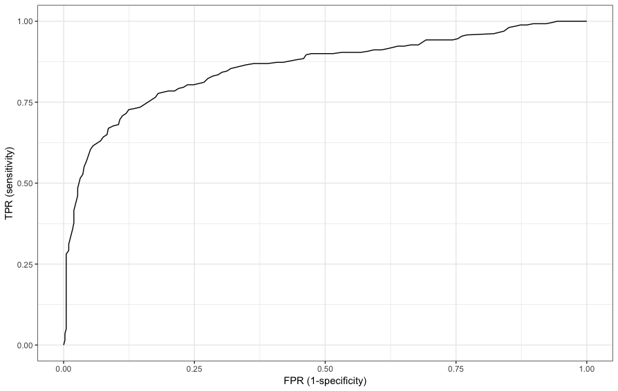
We can also obtain the AUC
> ml_log$summary$area_under_roc()
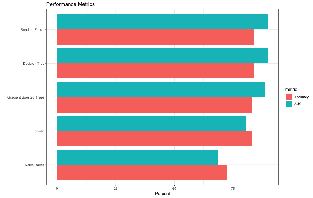
[1] 0.8575563Comparing prediction models
In this section we will run several Machine Learning algorithms:
- Logistic regression
> ptm=proc.time()
> ml_log <- ml_logistic_regression(train_tbl, ml_formula)
> x_log=proc.time()-ptm- Decision trees
> ptm=proc.time()
> ml_dt <- ml_decision_tree(train_tbl, ml_formula)
> x_dt=proc.time()-ptm- Random forest
> ptm=proc.time()
> ml_rf <- ml_random_forest(train_tbl, ml_formula)
> x_rf=proc.time()-ptm- Gradient boosted trees
> ptm=proc.time()
> ml_gbt <- ml_gradient_boosted_trees(train_tbl, ml_formula)
> x_gbt=proc.time()-ptm- Naive Bayes
> ptm=proc.time()
> ml_nb <- ml_naive_bayes(train_tbl, ml_formula)
> x_nb=proc.time()-ptm
Let’s first compare the running the times
> run_time=c(x_log[3],x_dt[3],x_rf[3],x_gbt[3],x_nb[3])
> d1=cbind.data.frame(Model=c("Logistic","DT","RF","GBT","Naive Bayes"),runTime=run_time)
> d1
        Model runTime
1    Logistic   3.293
2          DT   2.769
3          RF   2.322
4         GBT   6.708
5 Naive Bayes   2.100
Let’s then compute the ROC, the AUC and the Accuracy of each model and display the results
- we put the result of the estimation of the models in one
listobject
> ml_models <- list(
+   "Logistic" = ml_log,
+   "Decision Tree" = ml_dt,
+   "Random Forest" = ml_rf,
+   "Gradient Boosted Trees" = ml_gbt,
+   "Naive Bayes" = ml_nb
+ )- We create a function for scoring
> score_test_data <- function(model, data=test_tbl){
+   pred <- ml_predict(model, data)
+   select(pred, Survived, prediction)
+ }- Score all the models
> ml_score_test <- lapply(ml_models, score_test_data)Though ROC curves are not available in Spark, we need then to program them.
- This is a function that computes the accuracy
> calc_accuracy <- function(data, cutpoint = 0.5){
+   data %>%
+     mutate(prediction = if_else(prediction > cutpoint, 1.0, 0.0)) %>%
+     ml_multiclass_classification_evaluator("prediction", "Survived", "accuracy")
+ }- Calculate AUC and accuracy
> perf_metrics <- data.frame(
+   model = names(ml_score_test),
+   AUC = 100 * sapply(ml_score_test, ml_binary_classification_evaluator, "Survived", "prediction"),
+   Accuracy = 100 * sapply(ml_score_test, calc_accuracy),
+ row.names = NULL, stringsAsFactors = FALSE)- Plot the results
> gather(perf_metrics, metric, value, AUC, Accuracy) %>%
+   ggplot(aes(reorder(model, value), value, fill = metric)) +
+   geom_bar(stat = "identity", position = "dodge") +
+   coord_flip() +
+   xlab("") +
+   ylab("Percent") +
+   ggtitle("Performance Metrics")+theme_bw()